IRDA soil data
By Johanie Fournier, agr. in rstats tidyverse
October 23, 2023
IRDA here in Quebec, is generous enough to put on their website all the data from their soil studies. You can find it here
I download all of it on my computer and you can find the process in this github repro.
Now, let’s see what we got in this data set!
Get the data
Let’s look at the data of Chaudière-Appalaches
board_prepared <- pins::board_folder(path_to_file, versioned = TRUE)

data <- board_prepared %>%
  pins::pin_read("TS_chaudiere_appalaches")
Explore the data
There is a lot of information in there!! I usually go directly to the most interesting part: the texture, but let’s explore a bit more here.
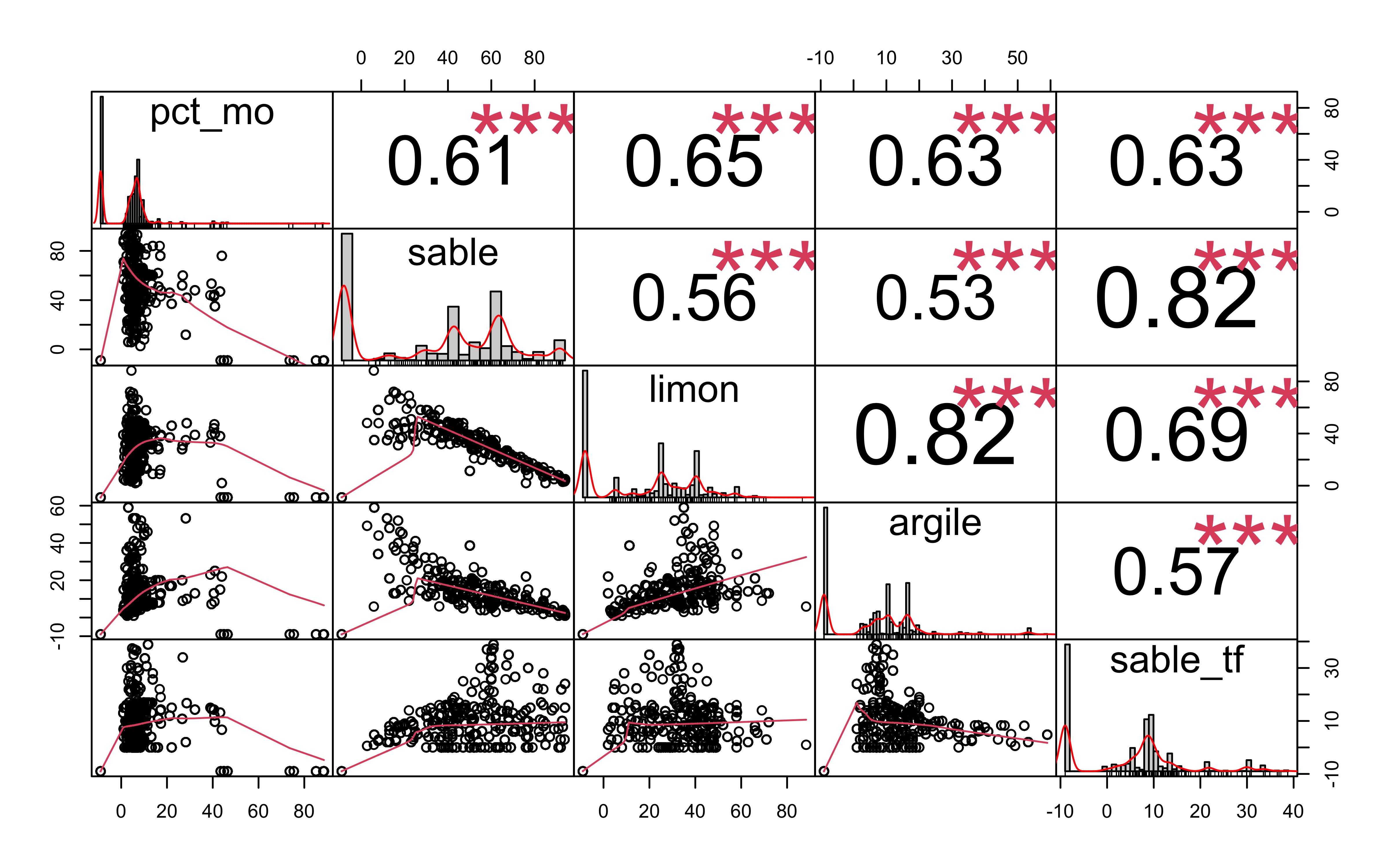
Let’s see how everything is correlated.
data %>%
  select(pct_mo, sable, limon, argile, sable_tf) %>%
  mutate_all(as.numeric) %>%
  drop_na() %>%
  my_corr_num_graph(data)
## NULL
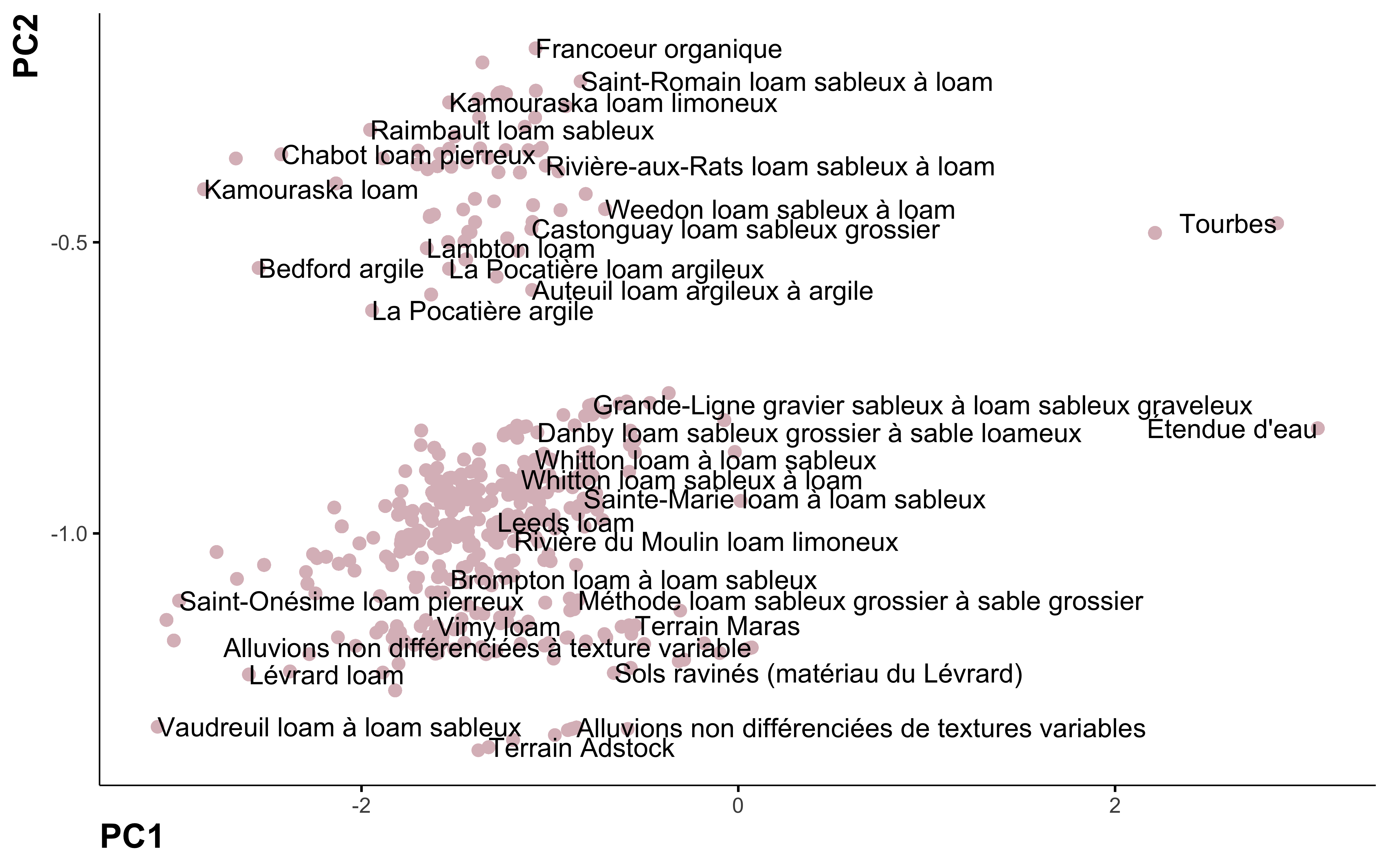
Principal component analysis
Let’s do a bit dimentionnality reduction!
step_pca
data_pca <- data %>%
  select(nom_sol, pct_mo, sable, limon, argile, sable_tf, clas_react, clas_calca, clas_humid) %>%
  mutate_at(c("pct_mo", "sable", "limon", "argile", "sable_tf"), as.numeric) %>%
  mutate_at(c("clas_react", "clas_calca", "clas_humid"), as.factor) %>%
  drop_na()
pca <- recipe(~., data = data_pca) %>%
  update_role(nom_sol, new_role = "id") %>%
  step_normalize(all_numeric_predictors()) %>%
  step_dummy(all_nominal_predictors()) %>%
  step_pca(all_predictors()) %>%
  prep() %>%
  bake(., new_data = NULL)


pca %>%
  ggplot(aes(PC1, PC2, label = nom_sol)) +
  geom_point(color = "#DBBDC3", size = 2) +
  geom_text(check_overlap = TRUE, hjust = "inward") +
  labs(color = NULL)
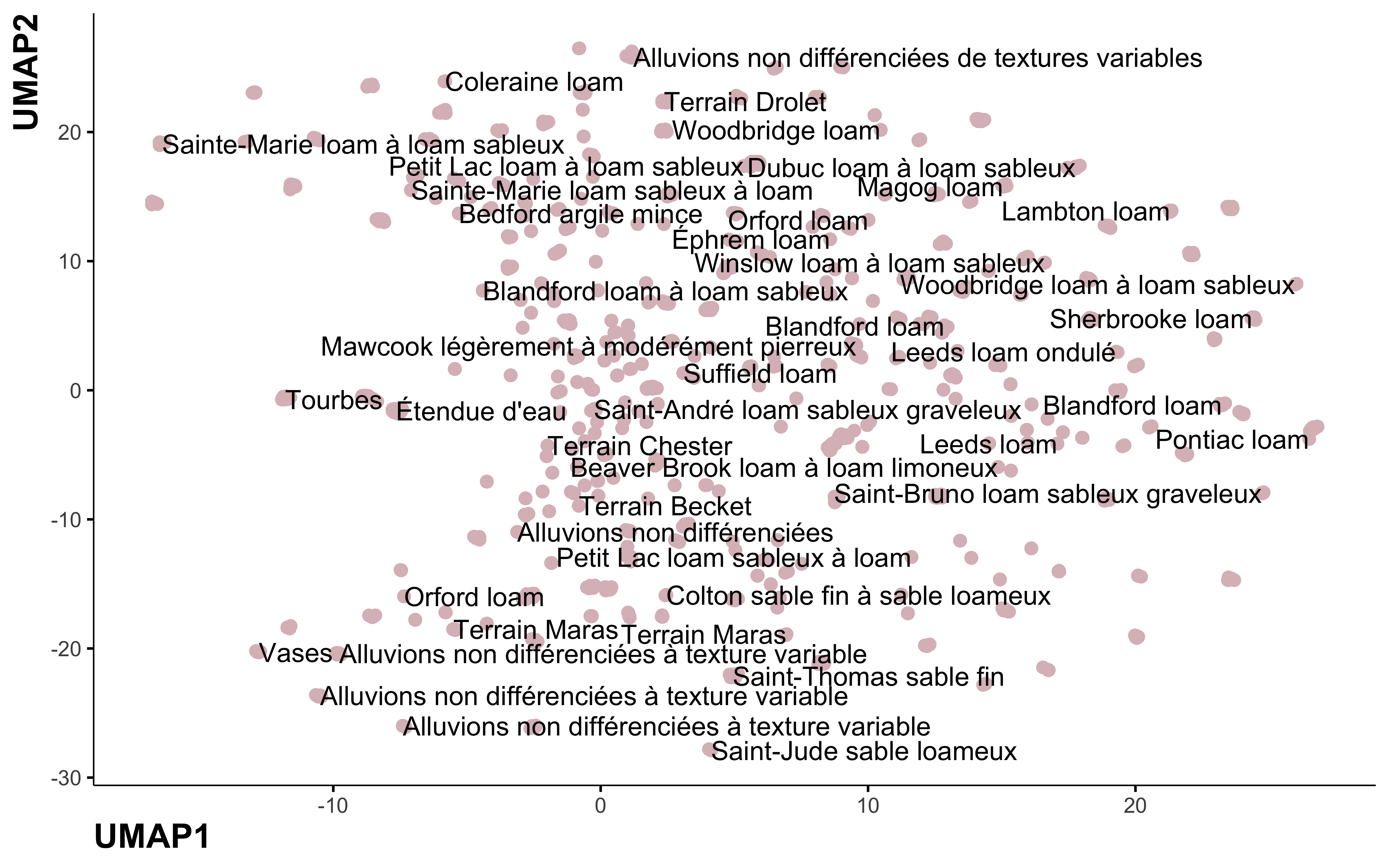
step_umap
library(embed)

umap_pca <- recipe(~., data = data_pca) %>%
  update_role(nom_sol, new_role = "id") %>%
  step_normalize(all_numeric_predictors()) %>%
  step_dummy(all_nominal_predictors()) %>%
  step_umap(all_predictors()) %>%
  prep() %>%
  bake(., new_data = NULL)

umap_pca %>%
  ggplot(aes(UMAP1, UMAP2, label = nom_sol)) +
  geom_point(color = "#DBBDC3", size = 2) +
  geom_text(check_overlap = TRUE, hjust = "inward") +
  labs(color = NULL)
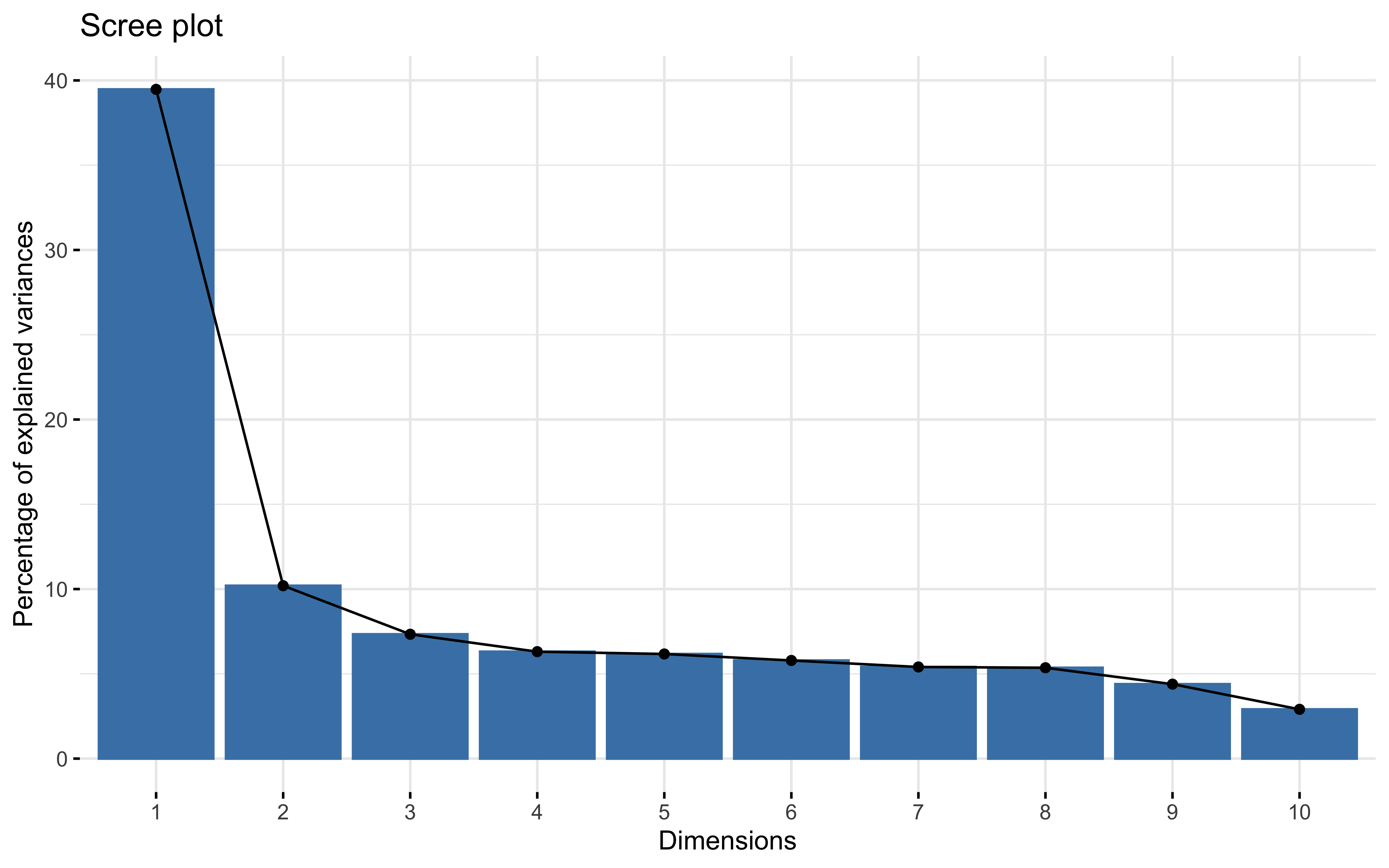
prcomp
Test 1
prcomp_pca <- recipe(~., data = data_pca) %>%
  update_role(nom_sol, new_role = "id") %>%
  step_normalize(all_numeric_predictors()) %>%
  step_dummy(all_nominal_predictors()) %>%
  prep() %>%
  bake(., new_data = NULL) %>%
  select(-nom_sol) %>%
  prcomp(., tol = 0.1, scale = TRUE)

prcomp_pca %>%
  summary(prcomp_pca)
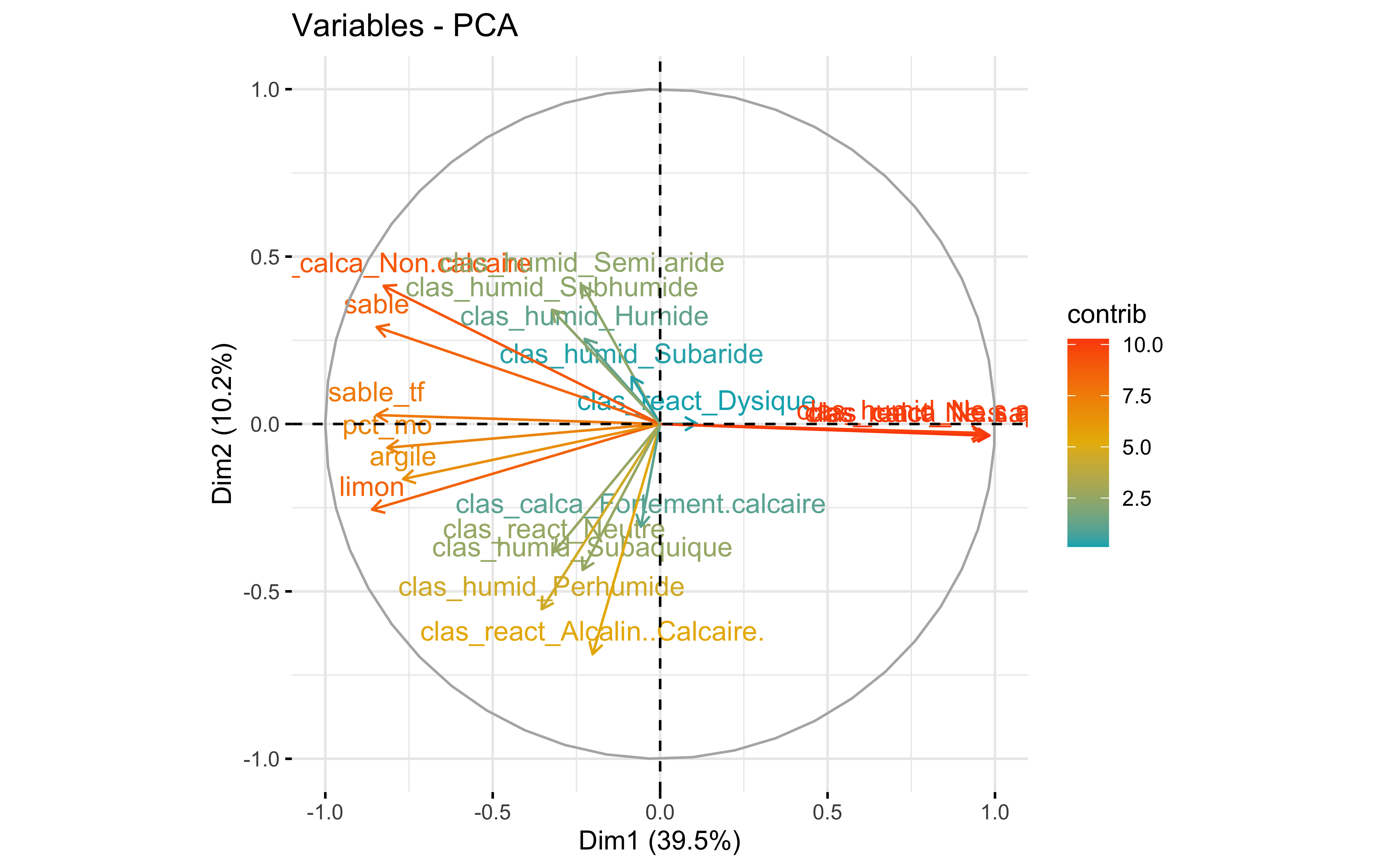
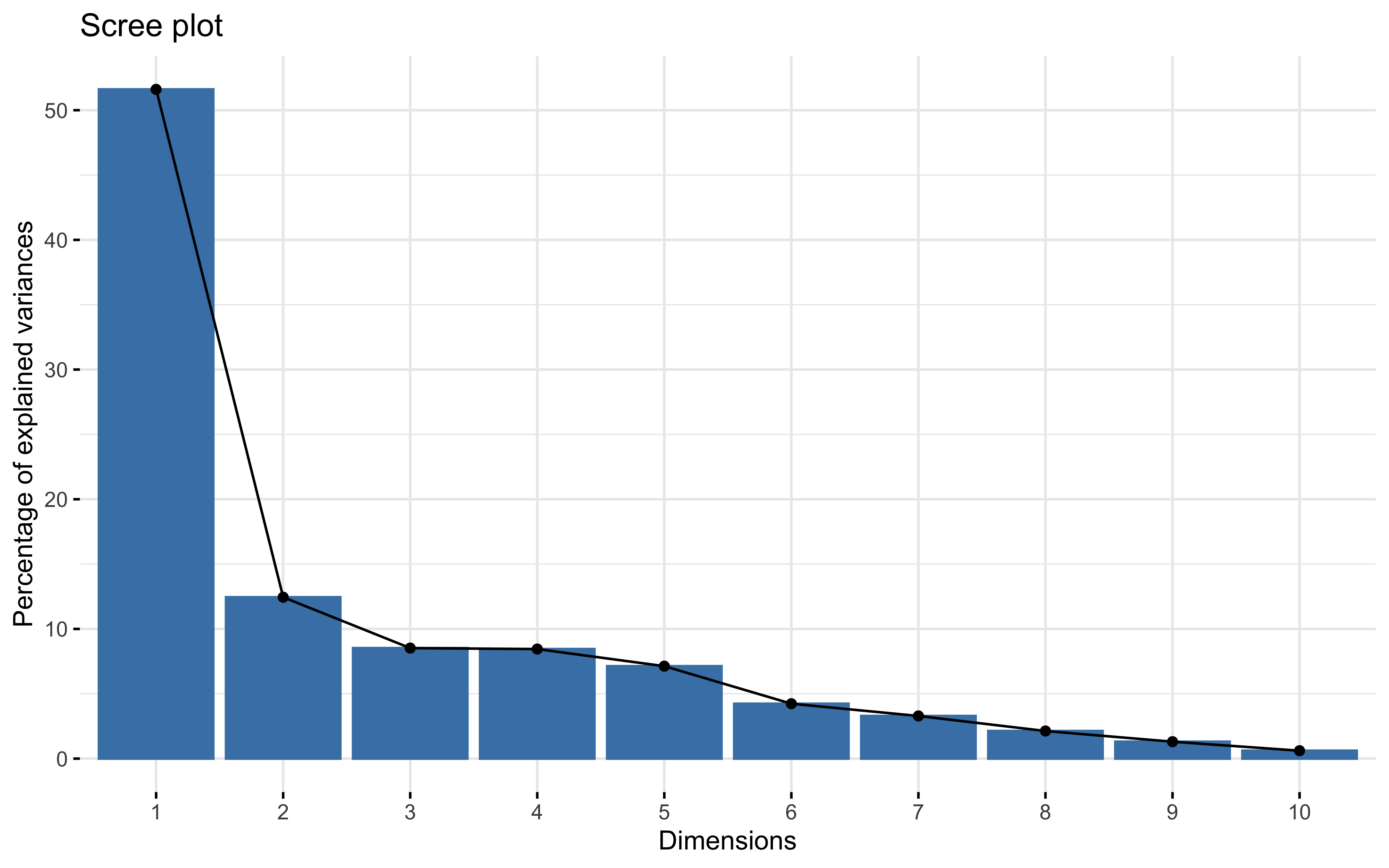
## Importance of first k=14 (out of 19) components:
##                           PC1    PC2     PC3     PC4     PC5     PC6     PC7
## Standard deviation     2.7386 1.3919 1.18051 1.09472 1.08282 1.04870 1.01337
## Proportion of Variance 0.3947 0.1020 0.07335 0.06307 0.06171 0.05788 0.05405
## Cumulative Proportion  0.3947 0.4967 0.57005 0.63312 0.69483 0.75271 0.80676
##                            PC8     PC9    PC10    PC11    PC12    PC13    PC14
## Standard deviation     1.00904 0.91347 0.74312 0.62665 0.56573 0.51546 0.35904
## Proportion of Variance 0.05359 0.04392 0.02906 0.02067 0.01684 0.01398 0.00678
## Cumulative Proportion  0.86035 0.90427 0.93333 0.95400 0.97084 0.98483 0.99161
factoextra::fviz_eig(prcomp_pca)
factoextra::fviz_pca_var(prcomp_pca,
  col.var = "contrib",
  gradient.cols = c("#00AFBB", "#E7B800", "#FC4E07")
)
Test 2
data_pca_smpl <- data_pca %>%
  select(-clas_humid)

prcomp_pca <- recipe(~., data = data_pca_smpl) %>%
  update_role(nom_sol, new_role = "id") %>%
  step_normalize(all_numeric_predictors()) %>%
  step_dummy(all_nominal_predictors()) %>%
  prep() %>%
  bake(., new_data = NULL) %>%
  select(-nom_sol) %>%
  prcomp(., tol = 0.1, scale = TRUE)

summary(prcomp_pca)
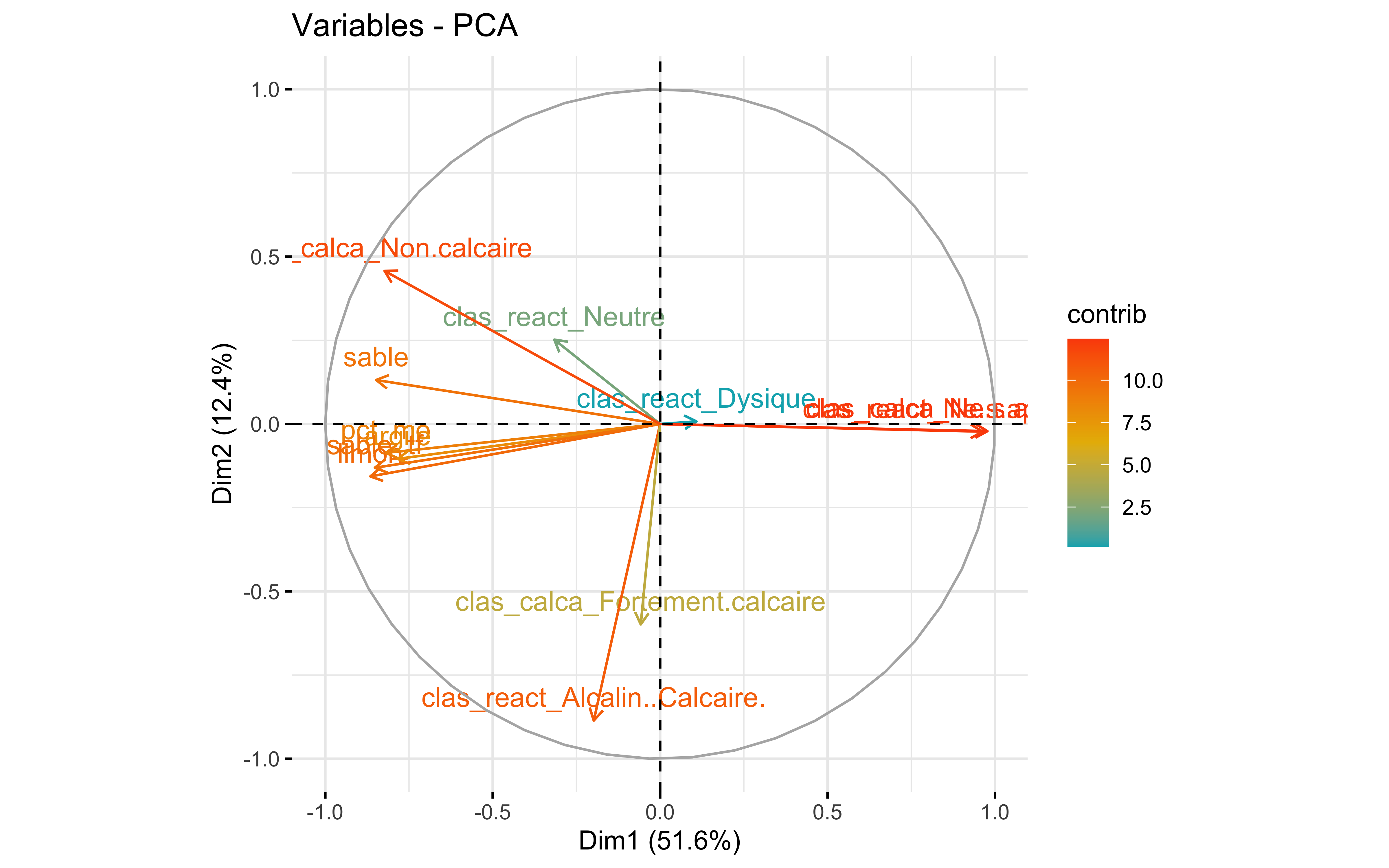
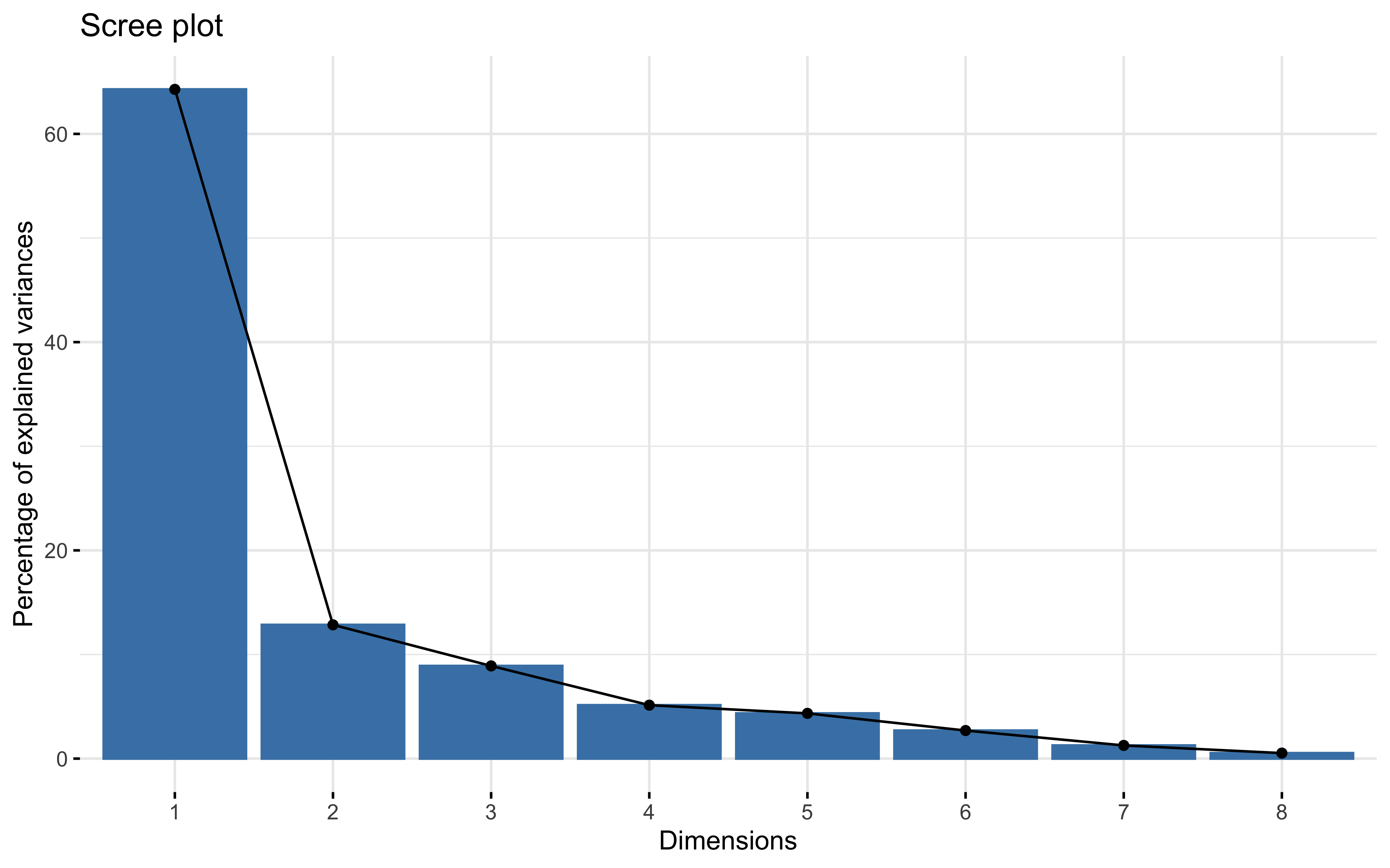
## Importance of first k=10 (out of 12) components:
##                           PC1    PC2     PC3     PC4     PC5     PC6     PC7
## Standard deviation     2.4885 1.2221 1.01127 1.00687 0.92494 0.71271 0.62815
## Proportion of Variance 0.5161 0.1245 0.08522 0.08448 0.07129 0.04233 0.03288
## Cumulative Proportion  0.5161 0.6405 0.72574 0.81022 0.88151 0.92384 0.95672
##                            PC8     PC9   PC10
## Standard deviation     0.50548 0.39574 0.2706
## Proportion of Variance 0.02129 0.01305 0.0061
## Cumulative Proportion  0.97802 0.99107 0.9972
factoextra::fviz_eig(prcomp_pca)
factoextra::fviz_pca_var(prcomp_pca,
  col.var = "contrib",
  gradient.cols = c("#00AFBB", "#E7B800", "#FC4E07")
)
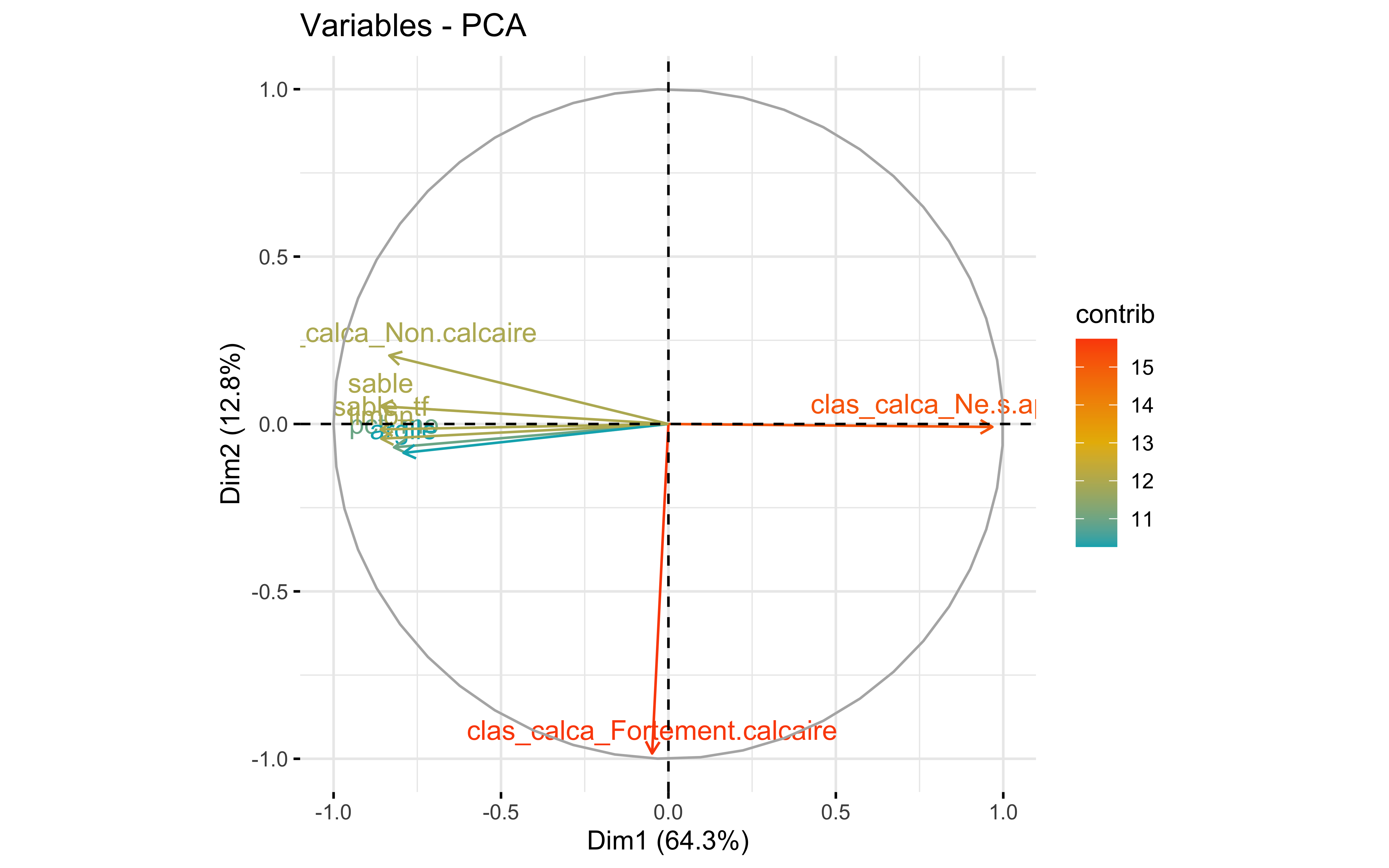
Test 3
data_pca_smpl <- data_pca %>%
  select(-clas_humid, -clas_react)

prcomp_pca <- recipe(~., data = data_pca_smpl) %>%
  update_role(nom_sol, new_role = "id") %>%
  step_normalize(all_numeric_predictors()) %>%
  step_dummy(all_nominal_predictors()) %>%
  prep() %>%
  bake(., new_data = NULL) %>%
  select(-nom_sol) %>%
  prcomp(., tol = 0.1, scale = TRUE)

summary(prcomp_pca)
## Importance of first k=7 (out of 8) components:
##                           PC1    PC2     PC3     PC4     PC5     PC6     PC7
## Standard deviation     2.2676 1.0138 0.84391 0.64084 0.58962 0.46451 0.31824
## Proportion of Variance 0.6428 0.1285 0.08902 0.05133 0.04346 0.02697 0.01266
## Cumulative Proportion  0.6428 0.7713 0.86028 0.91162 0.95507 0.98204 0.99470
factoextra::fviz_eig(prcomp_pca)
factoextra::fviz_pca_var(prcomp_pca,
  col.var = "contrib",
  gradient.cols = c("#00AFBB", "#E7B800", "#FC4E07")
)
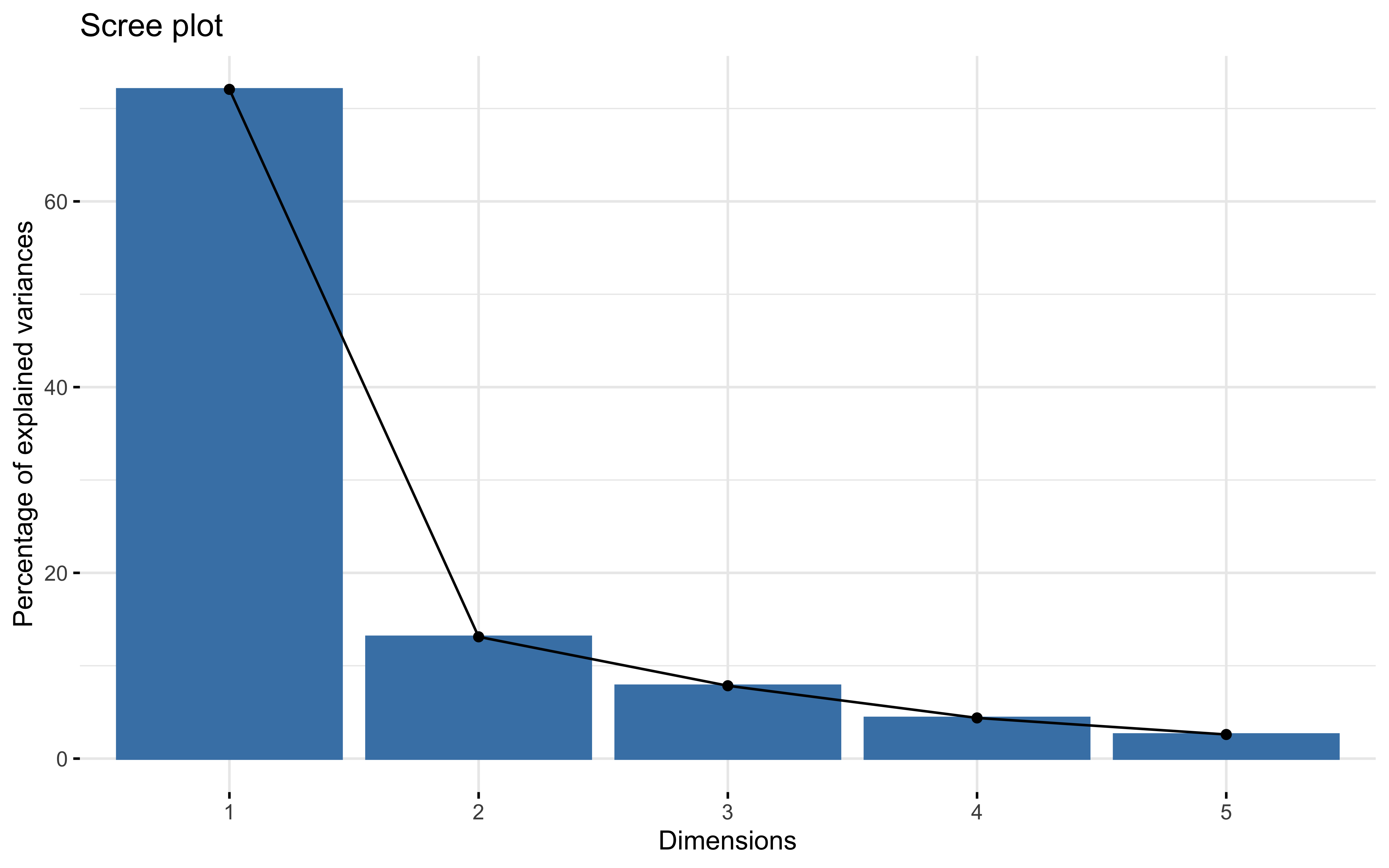
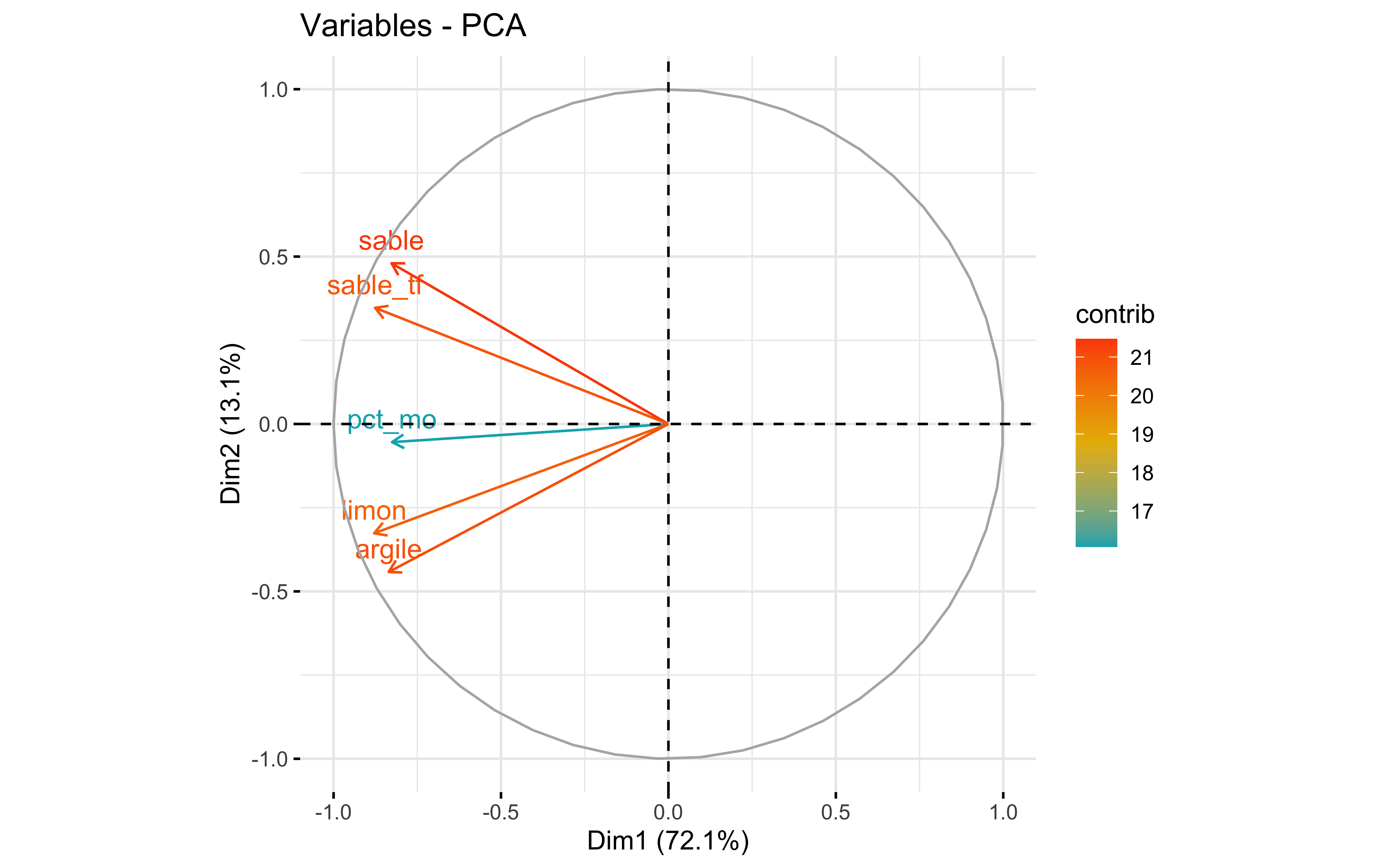
Test 4
data_pca_smpl <- data_pca %>%
  select(-clas_humid, -clas_react, -clas_calca)

prcomp_pca <- recipe(~., data = data_pca_smpl) %>%
  update_role(nom_sol, new_role = "id") %>%
  step_normalize(all_numeric_predictors()) %>%
  step_dummy(all_nominal_predictors()) %>%
  prep() %>%
  bake(., new_data = NULL) %>%
  select(-nom_sol) %>%
  prcomp(., tol = 0.1, scale = TRUE)

summary(prcomp_pca)
## Importance of components:
##                           PC1    PC2     PC3     PC4     PC5
## Standard deviation     1.8982 0.8097 0.62634 0.46801 0.36039
## Proportion of Variance 0.7206 0.1311 0.07846 0.04381 0.02598
## Cumulative Proportion  0.7206 0.8518 0.93022 0.97402 1.00000
factoextra::fviz_eig(prcomp_pca)
factoextra::fviz_pca_var(prcomp_pca,
  col.var = "contrib",
  gradient.cols = c("#00AFBB", "#E7B800", "#FC4E07")
)
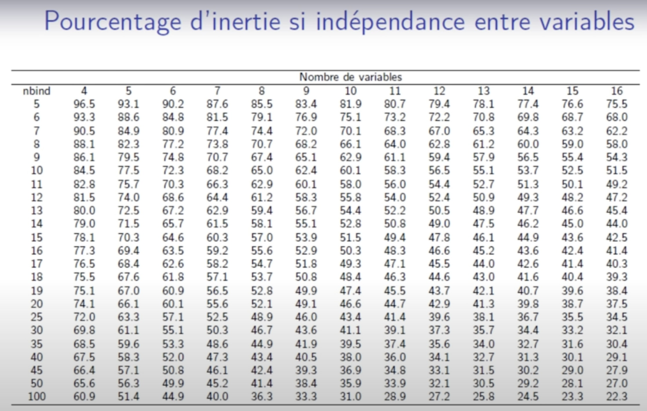
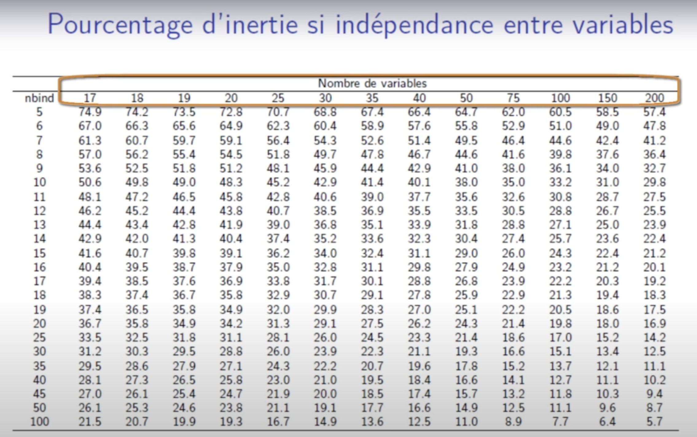
Percentage of variance obtain under independence 1:
- Posted on:
- October 23, 2023
- Length:
- 4 minute read, 715 words