TyT2019W34 - Stack of Histograms
By Johanie Fournier, agr. in rstats tidyverse tidytuesday
August 20, 2019
Get the data
nuclear_explosions <- readr::read_csv("https://raw.githubusercontent.com/rfordatascience/tidytuesday/master/data/2019/2019-08-20/nuclear_explosions.csv")
## Rows: 2051 Columns: 16
## ── Column specification ────────────────────────────────────────────────────────
## Delimiter: ","
## chr  (6): country, region, source, purpose, name, type
## dbl (10): date_long, year, id_no, latitude, longitude, magnitude_body, magni...
##
## ℹ Use `spec()` to retrieve the full column specification for this data.
## ℹ Specify the column types or set `show_col_types = FALSE` to quiet this message.
Explore the data
summary(nuclear_explosions)
##    date_long             year          id_no         country
##  Min.   :19450716   Min.   :1945   Min.   :45001   Length:2051
##  1st Qu.:19621066   1st Qu.:1962   1st Qu.:62140   Class :character
##  Median :19700501   Median :1970   Median :70021   Mode  :character
##  Mean   :19709736   Mean   :1971   Mean   :70934
##  3rd Qu.:19790920   3rd Qu.:1979   3rd Qu.:79044
##  Max.   :19980530   Max.   :1998   Max.   :98005
##
##     region             source             latitude        longitude
##  Length:2051        Length:2051        Min.   :-49.50   Min.   :-169.32
##  Class :character   Class :character   1st Qu.: 37.00   1st Qu.:-116.05
##  Mode  :character   Mode  :character   Median : 37.10   Median :-116.00
##                                        Mean   : 35.40   Mean   : -36.05
##                                        3rd Qu.: 49.87   3rd Qu.:  78.00
##                                        Max.   : 75.10   Max.   : 179.22
##
##  magnitude_body  magnitude_surface     depth            yield_lower
##  Min.   :0.000   Min.   :0.0000    Min.   :-400.0000   Min.   :    0.0
##  1st Qu.:0.000   1st Qu.:0.0000    1st Qu.:   0.0000   1st Qu.:    0.0
##  Median :0.000   Median :0.0000    Median :   0.0000   Median :    0.0
##  Mean   :2.145   Mean   :0.3558    Mean   :  -0.4896   Mean   :  209.2
##  3rd Qu.:5.100   3rd Qu.:0.0000    3rd Qu.:   0.0000   3rd Qu.:   20.0
##  Max.   :7.400   Max.   :6.0000    Max.   :   1.4510   Max.   :50000.0
##                                                        NA's   :3
##   yield_upper         purpose              name               type
##  Min.   :    0.00   Length:2051        Length:2051        Length:2051
##  1st Qu.:   18.25   Class :character   Class :character   Class :character
##  Median :   20.00   Mode  :character   Mode  :character   Mode  :character
##  Mean   :  323.43
##  3rd Qu.:  150.00
##  Max.   :50000.00
##  NA's   :5
Prepare the data
#quel est le pays qui enregistre le plus d'explosion nucléaire?
nuclear_explosions_cat <- nuclear_explosions %>%
  inspect_cat()
pct_country<-nuclear_explosions_cat$levels$country %>%
  mutate(type="country")
#rep=USA avec 50%

#Dans quel région les États-Unis font-ils exploser leurs bombes?
nuclear_explosions_cat <- nuclear_explosions %>%
  filter(country=="USA") %>%
  inspect_cat()
pct_region<-nuclear_explosions_cat$levels$region %>%
  mutate(type="country")
#rep: NTS avec 88% (Nevada Test Site)

#Pour quel raison?
nuclear_explosions_cat <- nuclear_explosions %>%
  filter(country=="USA") %>%
  mutate(raison="autres") %>%
  mutate(raison=ifelse(purpose=="COMBAT", "COMBAT", raison)) %>%
  mutate(raison=ifelse(purpose %in% c("WR", "WE", "WE/WR", "WR/WE", "SE/WR", "WR/SE"), "Training", raison)) %>%
  inspect_cat()
pct_purpose<-nuclear_explosions_cat$levels$purpose
pct_purpose<-nuclear_explosions_cat$levels$raison %>%
  mutate(type="country")
Visualize the data
#Graphique 1: Qui
gg<-ggplot(pct_country, aes(x=type, y=prop, fill=reorder(value, -prop)))
gg <- gg + geom_chicklet(width = 1.8)
gg <- gg + coord_flip()
gg <- gg + scale_fill_manual(values=c("#749594", "#AFB7BB", "#AFB7BB", "#AFB7BB", "#AFB7BB", "#AFB7BB", "#AFB7BB"))
#retirer la légende
gg <- gg + theme(legend.position = "none")
#ajuster les axes
gg <- gg + expand_limits(y=c(0, 1.3))
gg <- gg + expand_limits(x=c(-4, 3))
#modifier le thème
gg <- gg + theme(panel.border = element_blank(),
panel.background = element_blank(),
plot.background = element_blank(),
panel.grid.major.x= element_blank(),
panel.grid.major.y= element_blank(),
panel.grid.minor = element_blank(),
axis.line.x = element_blank(),
axis.line.y = element_blank(),
axis.ticks.y = element_blank(),
axis.ticks.x = element_blank())
#ajouter les titres
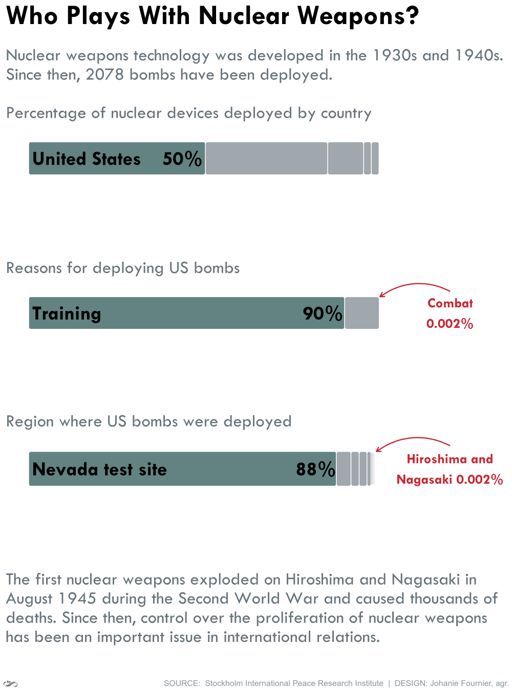
gg<-gg + labs(title="Who Plays With Nuclear Weapons?",
subtitle="\nNuclear weapons technology was developed in the 1930s and 1940s.\nSince then, 2078 bombs have been deployed.\n\nPercentage of nuclear devices deployed by country",
y=" ",
x=" ")
gg<-gg + theme(plot.title = element_text(size=40, hjust=0,vjust=0, face="bold", family="Tw Cen MT"),
plot.subtitle = element_text(size=25, hjust=0,vjust=0, family="Tw Cen MT", color="#7A878E"),
axis.title.y = element_blank(),
axis.title.x = element_blank(),
axis.text.y = element_blank(),
axis.text.x = element_blank())
#ajouter les étiquettes de données
gg<-gg + annotate(geom="text", x=1,y=0.01, label="United States", color="black", size=10, hjust=0,vjust=0.5, fontface="bold", family="Tw Cen MT")
gg<-gg + annotate(geom="text", x=1,y=0.38, label="50%", color="black", size=10, hjust=0,vjust=0.5, fontface="bold", family="Tw Cen MT")
#Graphique 2: pourquoi
gg<-ggplot(pct_purpose, aes(x=type, y=prop))
gg <- gg + geom_chicklet(aes(fill=reorder(value, -prop)),width = 1.8)
gg <- gg + coord_flip()
gg <- gg + scale_fill_manual(values=c("#749594", "#AFB7BB", "#AFB7BB"))
#retirer la légende
gg <- gg + theme(legend.position = "none")
#ajuster les axes
gg <- gg + expand_limits(y=c(0, 1.3))
gg <- gg + expand_limits(x=c(-4, 3))
#modifier le thème
gg <- gg + theme(panel.border = element_blank(),
panel.background = element_blank(),
plot.background = element_blank(),
panel.grid.major.x= element_blank(),
panel.grid.major.y= element_blank(),
panel.grid.minor = element_blank(),
axis.line.x = element_blank(),
axis.line.y = element_blank(),
axis.ticks.y = element_blank(),
axis.ticks.x = element_blank())
#ajouter les titres
gg<-gg + labs(title=" ",
subtitle="Reasons for deploying US bombs",
y=" ",
x=" ")
gg<-gg + theme(plot.title = element_blank(),
plot.subtitle = element_text(size=25, hjust=0,vjust=0, family="Tw Cen MT", color="#7A878E"),
axis.title.y = element_blank(),
axis.title.x = element_blank(),
axis.text.y = element_blank(),
axis.text.x = element_blank())
#Faire des flèches
arrows <- tibble(
x1 = c(2.2),
x2 = c(1.9),
y1 = c(1.20),
y2 = c(1)
)
gg<-gg + geom_curve(data = arrows, aes(x = x1, y = y1, xend = x2, yend = y2),
arrow = arrow(length = unit(0.1, "inch")),
size = 0.8, color = "#D33E43", curvature = 0.3)
#ajouter les étiquettes de données
gg<-gg + annotate(geom="text", x=1,y=0.01, label="Training", color="black", size=10, hjust=0,vjust=0.5, fontface="bold", family="Tw Cen MT")
gg<-gg + annotate(geom="text", x=1,y=0.78, label="90%", color="black", size=10, hjust=0,vjust=0.5, fontface="bold", family="Tw Cen MT")
gg<-gg + annotate(geom="text", x=1,y=1.2, label="Combat\n0.002%", color="#D33E43", size=7, hjust=0.5,vjust=0.5, fontface="bold", family="Tw Cen MT")
#Graphique 3: ou
gg<-ggplot(pct_region, aes(x=type, y=prop))
gg <- gg + geom_chicklet(aes(fill=reorder(value, -prop)),width = 1.8)
gg <- gg + coord_flip()
gg <- gg + scale_fill_manual(values=c("#749594", "#AFB7BB", "#AFB7BB", "#AFB7BB", "#AFB7BB", "#AFB7BB", "#AFB7BB", "#AFB7BB", "#AFB7BB", "#AFB7BB", "#AFB7BB", "#AFB7BB", "#AFB7BB", "#AFB7BB", "#AFB7BB", "#AFB7BB", "#AFB7BB", "#AFB7BB", "#AFB7BB", "#AFB7BB", "#AFB7BB", "#AFB7BB", "#AFB7BB"))
#retirer la légende
gg <- gg + theme(legend.position = "none")
#ajuster les axes
gg <- gg + expand_limits(y=c(0, 1.3))
gg <- gg + expand_limits(x=c(-4, 3))
#modifier le thème
gg <- gg + theme(panel.border = element_blank(),
panel.background = element_blank(),
plot.background = element_blank(),
panel.grid.major.x= element_blank(),
panel.grid.major.y= element_blank(),
panel.grid.minor = element_blank(),
axis.line.x = element_blank(),
axis.line.y = element_blank(),
axis.ticks.y = element_blank(),
axis.ticks.x = element_blank())
#ajouter les titres
gg<-gg + labs(title=" ",
subtitle="Region where US bombs were deployed",
y=" ",
x=" ",
caption= "The first nuclear weapons exploded on Hiroshima and Nagasaki in\nAugust 1945 during the Second World War and caused thousands of\ndeaths. Since then, control over the proliferation of nuclear weapons\nhas been an important issue in international relations.\n")
gg<-gg + theme(plot.title = element_blank(),
plot.subtitle = element_text(size=25, hjust=0,vjust=0, family="Tw Cen MT", color="#7A878E"),
plot.caption = element_text(size=25, hjust=0,vjust=0, family="Tw Cen MT", color="#7A878E"),
axis.title.y = element_blank(),
axis.title.x = element_blank(),
axis.text.y = element_blank(),
axis.text.x = element_blank())
#Faire des flèches
arrows <- tibble(
x1 = c(2.2),
x2 = c(1.9),
y1 = c(1.20),
y2 = c(0.99)
)
gg<-gg + geom_curve(data = arrows, aes(x = x1, y = y1, xend = x2, yend = y2),
arrow = arrow(length = unit(0.1, "inch")),
size = 0.8, color = "#D33E43", curvature = 0.3)
#ajouter les étiquettes de données
gg<-gg + annotate(geom="text", x=1,y=0.01, label="Nevada test site", color="black", size=10, hjust=0,vjust=0.5, fontface="bold", family="Tw Cen MT")
gg<-gg + annotate(geom="text", x=1,y=0.76, label="88%", color="black", size=10, hjust=0,vjust=0.5, fontface="bold", family="Tw Cen MT")
gg<-gg + annotate(geom="text", x=1,y=1.2, label="Hiroshima and\nNagasaki 0.002%", color="#D33E43", size=7, hjust=0.5,vjust=0.5, fontface="bold", family="Tw Cen MT")
- Posted on:
- August 20, 2019
- Length:
- 6 minute read, 1075 words
- Categories:
- rstats tidyverse tidytuesday
- Tags:
- rstats tidyverse tidytuesday