TyT2019W36 - Mix and Match

cpu <- readr::read_csv("https://raw.githubusercontent.com/rfordatascience/tidytuesday/master/data/2019/2019-09-03/cpu.csv")

summary(cpu)

#Quel est la moyenne de 2018?
moy_2018<-cpu %>% 
  mutate(transistor_count=as.numeric(transistor_count)) %>% 
  filter(date_of_introduction==2018) %>% 
  summarise(mean=mean(transistor_count, na.rm =TRUE))
#rep: 9898250000

#Qui sont les desinger encore présent en 2018?
desinger_2018<-cpu %>% 
  mutate(transistor_count=as.numeric(transistor_count)) %>% 
  filter(date_of_introduction==2018) 
#rep: Qualcomm, Apple, Fujitsu, Huawei,  Nvidia

#Quel est la valeur du processeur au début pour chaque desinger?
debut<-cpu %>%
   filter(designer %in% c("Qualcomm", "Apple", "Fujitsu", "Huawei", "Nvidia")& !is.na(transistor_count)) %>% 
    group_by(designer) %>%
    filter(date_of_introduction==min(date_of_introduction)) %>% 
    mutate(deb=transistor_count) %>% 
    select(deb, designer) %>% 
    ungroup()


#Quel est la valeur du processeur en 2018 pour chaque desinger?
fin<-cpu %>%
   filter(designer %in% c("Qualcomm", "Apple", "Fujitsu", "Huawei", "Nvidia") & !is.na(transistor_count)) %>% 
    group_by(designer) %>%
    filter(transistor_count==max(transistor_count)) %>% 
    mutate(last=transistor_count) %>% 
    select(last, designer) %>% 
    ungroup()


#Mettre tout dans une même base de donnée
data<-debut %>% 
  left_join(fin) %>% 
  mutate(moy_2018=9898.25) %>% 
  mutate(max=2*9898.25)

#Graphique
gg<-ggplot(data, aes(x=designer, y=max))
gg <- gg + geom_chicklet(width=0.45, radius=grid::unit(10, "pt"), fill="#F7F7F7")
gg <- gg + geom_errorbar(aes(y=moy_2018, x=designer, ymin=moy_2018, ymax=moy_2018), color="black", width=0.45, size=1.5) 
#debut
gg <- gg +  geom_text(aes(y = 1.00e+03, x = 1),label = "◀", size = 7, family = "HiraKakuPro-W3",  color="#FB8B24")
gg <- gg +  geom_text(aes(y = 0.110, x = 2),label = "◀", size = 7, family = "HiraKakuPro-W3", color="#FB8B24")
gg <- gg +  geom_text(aes(y = 4.00e+03, x = 3),label = "◀", size = 7, family = "HiraKakuPro-W3", color="#FB8B24")
gg <- gg +  geom_text(aes(y = 9.00e+03, x = 4),label = "◀", size = 7, family = "HiraKakuPro-W3", color="#FB8B24")
gg <- gg +  geom_text(aes(y = 3.00e+03, x = 5),label = "◀", size = 7, family = "HiraKakuPro-W3", color="#FB8B24")
#fin
gg <- gg +  geom_text(aes(y = 1.000e+04, x = 1),label = "▶", size = 7, family = "HiraKakuPro-W3", color="#FB8B24")
gg <- gg +  geom_text(aes(y = 8.786e+03, x = 2),label = "▶", size = 7, family = "HiraKakuPro-W3", color="#FB8B24")
gg <- gg +  geom_text(aes(y = 6.900e+03, x = 3),label = "▶", size = 7, family = "HiraKakuPro-W3", color="#FB8B24")
gg <- gg +  geom_text(aes(y = 9.000e+03, x = 4),label = "▶", size = 7, family = "HiraKakuPro-W3", color="#FB8B24")
gg <- gg +  geom_text(aes(y = 1.800e+04, x = 5),label = "▶", size = 7, family = "HiraKakuPro-W3", color="#FB8B24")
#Nom des desinger
gg <- gg +  geom_text(aes(y = 0, x = 1.5),label = "Apple", size = 7, hjust=0,family = "Tw Cen MT", color="#F7F7F7")
gg <- gg +  geom_text(aes(y = 0, x = 2.5),label = "Fujitsu", size = 7, hjust=0,family = "Tw Cen MT", color="#F7F7F7")
gg <- gg +  geom_text(aes(y = 0, x = 3.5),label = "Huawei", size = 7, hjust=0,family = "Tw Cen MT", color="#F7F7F7")
gg <- gg +  geom_text(aes(y = 0, x = 4.5),label = "Nvidia", size = 7, hjust=0,family = "Tw Cen MT", color="#F7F7F7")
gg <- gg +  geom_text(aes(y = 0, x = 5.5),label = "Qualcomm", size = 7, hjust=0,family = "Tw Cen MT", color="#F7F7F7")
#Légende sur le graphique
gg <- gg +  geom_text(aes(y = 16300, x = 5),label = "2018", size = 4.5, hjust=0,family = "Tw Cen MT", color="#FB8B24")
gg <- gg +  geom_text(aes(y = 9898.25, x = 5.4),label = "2018 global mean", size = 4, hjust=0.5,family = "Tw Cen MT", color="black")
gg <- gg +  geom_text(aes(y = 3500, x = 5),label = "start", size = 4.5, hjust=0,family = "Tw Cen MT", color="#FB8B24")
gg<- gg + coord_flip()
#modifier le thème
gg <- gg +  theme(panel.border = element_blank(),
                    panel.background = element_rect(fill="#2F4253"),
                    plot.background = element_rect(fill ="#2F4253"),
                    panel.grid.major.x= element_blank(),
                    panel.grid.major.y= element_blank(),
                    panel.grid.minor = element_blank(),
                    axis.line.x = element_blank(),
                    axis.line.y = element_blank(),
                    axis.ticks.y = element_blank(),
                    axis.ticks.x = element_blank())
#ajouter les titres
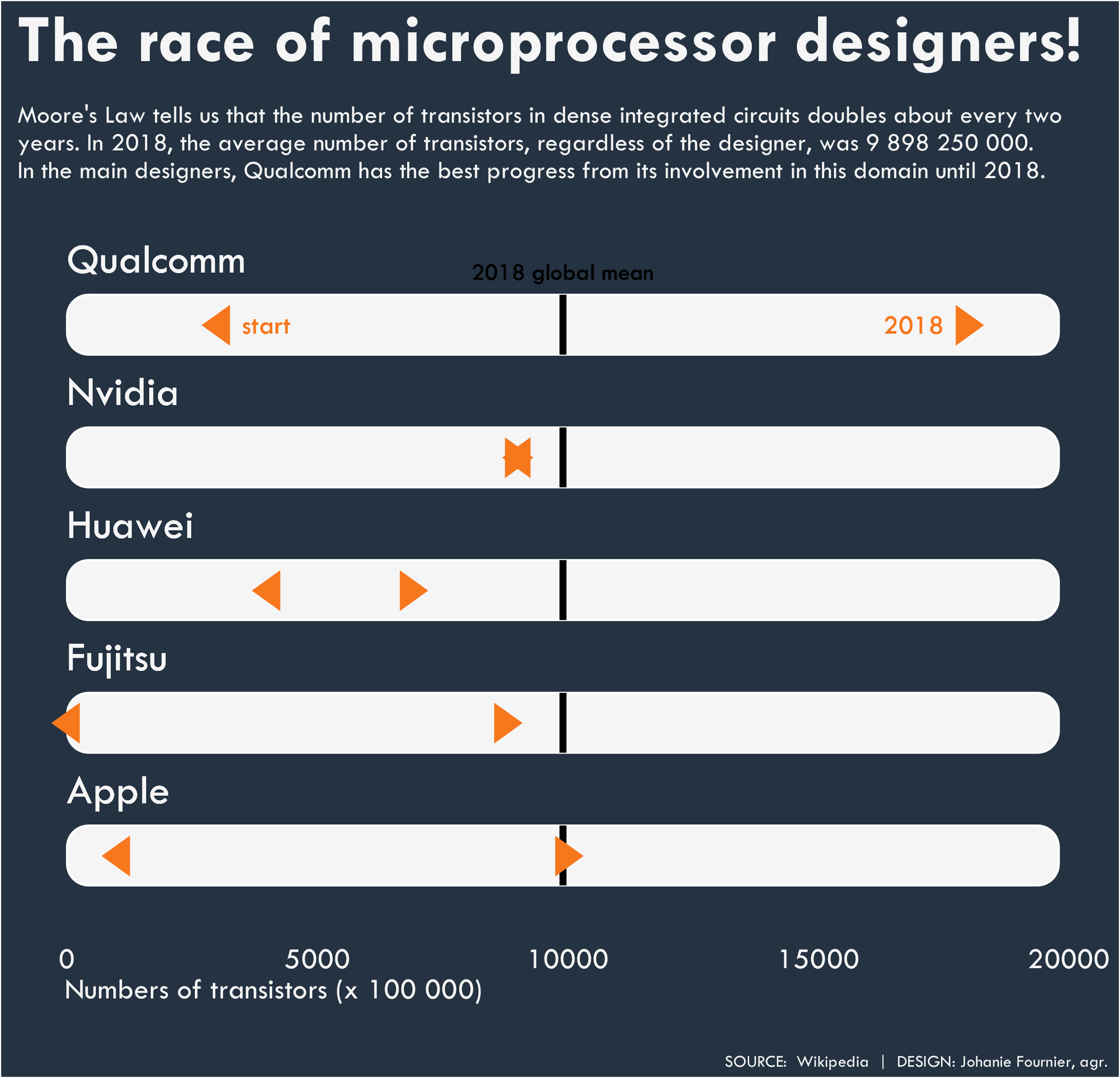
gg<-gg + labs(title="The race of microprocessor designers!",
              subtitle="\nMoore's Law tells us that the number of transistors in dense integrated circuits doubles about every two\nyears. In 2018, the average number of transistors, regardless of the designer, was 9 898 250 000.\nIn the main designers, Qualcomm has the best progress from its involvement in this domain until 2018.\n\n",
              y="Numbers of transistors (x 100 000)", 
              x=" ", 
              caption="\n\nSOURCE:  Wikipedia  |  DESIGN: Johanie Fournier, agr.")
gg<-gg + theme(plot.title      = element_text(size=32, hjust=0,vjust=0, face="bold", family="Tw Cen MT", color="#F7F7F7"),
                 plot.subtitle = element_text(size=12, hjust=0,vjust=0, family="Tw Cen MT", color="#F7F7F7"),
                 plot.caption =  element_text(size=8, hjust=1,vjust=0, family="Tw Cen MT", color="#F7F7F7"),
                 axis.title.y  = element_blank(),
                 axis.title.x  = element_text(size=14, hjust=0.07,vjust=0.5, family="Tw Cen MT", color="#F7F7F7"),
                 axis.text.x   = element_text(size=14, hjust=0.5,vjust=0.5, family="Tw Cen MT", color="#F7F7F7"), 
                 axis.text.y   = element_blank())