TyT2019W39 - Not a Real Graph
By Johanie Fournier, agr. in rstats tidyverse tidytuesday
September 25, 2019
Get the data
school_diversity <- readr::read_csv("https://raw.githubusercontent.com/rfordatascience/tidytuesday/master/data/2019/2019-09-24/school_diversity.csv")
## Rows: 27944 Columns: 15
## ── Column specification ────────────────────────────────────────────────────────
## Delimiter: ","
## chr (7): LEAID, LEA_NAME, ST, d_Locale_Txt, SCHOOL_YEAR, diverse, int_group
## dbl (8): AIAN, Asian, Black, Hispanic, White, Multi, Total, variance
##
## ℹ Use `spec()` to retrieve the full column specification for this data.
## ℹ Specify the column types or set `show_col_types = FALSE` to quiet this message.
Explore the data
summary(school_diversity)
##     LEAID             LEA_NAME              ST            d_Locale_Txt
##  Length:27944       Length:27944       Length:27944       Length:27944
##  Class :character   Class :character   Class :character   Class :character
##  Mode  :character   Mode  :character   Mode  :character   Mode  :character
##
##
##
##
##  SCHOOL_YEAR             AIAN              Asian              Black
##  Length:27944       Min.   :  0.0000   Min.   : 0.00000   Min.   :  0.0000
##  Class :character   1st Qu.:  0.0000   1st Qu.: 0.05818   1st Qu.:  0.2023
##  Mode  :character   Median :  0.1566   Median : 0.53124   Median :  0.9231
##                     Mean   :  2.7879   Mean   : 1.76956   Mean   :  6.5515
##                     3rd Qu.:  0.6144   3rd Qu.: 1.44514   3rd Qu.:  3.9649
##                     Max.   :100.0000   Max.   :74.90586   Max.   :100.0000
##
##     Hispanic            White            Multi            Total
##  Min.   :  0.0000   Min.   :  0.00   Min.   : 0.000   Min.   :      1
##  1st Qu.:  0.5505   1st Qu.: 65.24   1st Qu.: 1.070   1st Qu.:    366
##  Median :  2.7094   Median : 88.60   Median : 2.378   Median :   1044
##  Mean   : 10.4520   Mean   : 76.93   Mean   : 3.202   Mean   :   3228
##  3rd Qu.: 10.1256   3rd Qu.: 96.45   3rd Qu.: 4.174   3rd Qu.:   2720
##  Max.   :100.0000   Max.   :100.00   Max.   :85.308   Max.   :1020747
##                                      NA's   :14760
##    diverse             variance      int_group
##  Length:27944       Min.   :0.000   Length:27944
##  Class :character   1st Qu.:0.017   Class :character
##  Mode  :character   Median :0.046   Mode  :character
##                     Mean   :0.078
##                     3rd Qu.:0.107
##                     Max.   :0.601
##                     NA's   :24923
Prepare the data
school <- school_diversity %>%
  mutate(Abbreviation=ST) %>%
  left_join(code, by="Abbreviation") %>%
  mutate(code=case_when(diverse == 'Diverse' ~ 1,
                         diverse == 'Undiverse'  ~ 2,
                         diverse == 'Extremely undiverse'  ~ 3)) %>%
  mutate(annee=case_when(SCHOOL_YEAR == '1994-1995' ~ 1,
                         SCHOOL_YEAR == '2016-2017'  ~ 2)) %>%
  select("State", "annee", "code") %>%
  group_by(State, annee, code) %>%
  dplyr::summarise(freq=n()) %>%
  ungroup() %>%
  group_by(State, annee) %>%
  top_n(1,freq) %>%
  ungroup()

 rect_1 = data.frame(xmin = c(0.95,1.95),
                     xmax = c(1.05,2.05),
                     ymin = c(0.75,0.75),
                     ymax = c(1.25,1.25))

 rect_2 = data.frame(xmin = c(0.95,1.95),
                     xmax = c(1.05,2.05),
                     ymin = c(1.75,1.75),
                     ymax = c(2.25,2.25))

 rect_3 = data.frame(xmin = c(0.95,1.95),
                     xmax = c(1.05,2.05),
                     ymin = c(2.75,2.75),
                     ymax = c(3.25,3.25))

 school_1995<-school %>%
   filter(annee==1) %>%
   group_by(code) %>%
   dplyr::summarise(freq=n())

  school_2017<-school %>%
   filter(annee==2) %>%
   group_by(code) %>%
   dplyr::summarise(freq=n())
Visualize the data
#Graphique
gg<-ggplot(school, aes(x=annee, y=code, group=State, color=State))
gg<-gg + geom_line(position=position_jitter(w=0, h=0.1),size=1,color="#2E2E2E", alpha=0.5)
gg<-gg + geom_rect(data=rect_1, aes(xmin = xmin, xmax = xmax, ymin = ymin, ymax = ymax), color="#B494CC",fill = "#B494CC", inherit.aes=FALSE)
gg<-gg + geom_rect(data=rect_2, aes(xmin = xmin, xmax = xmax, ymin = ymin, ymax = ymax), color="#99C9DE",fill = "#99C9DE", inherit.aes=FALSE)
gg<-gg + geom_rect(data=rect_3, aes(xmin = xmin, xmax = xmax, ymin = ymin, ymax = ymax), color="#D1EAE5",fill = "#D1EAE5", inherit.aes=FALSE)
#ajuster les axes
gg<-gg + scale_x_continuous(breaks=seq(1,2,1), limits=c(0.8, 3), expand = c(0, 0), labels = c("1994-1995","2016-2017"))
#annoter
gg<-gg + annotate(geom="text", x=1,y=1, label="Diverse", color="#2E2E2E", size=4, hjust=0.5,vjust=0.5, fontface="bold", angle=90)
gg<-gg + annotate(geom="text", x=2,y=1, label="Diverse", color="#2E2E2E", size=4, hjust=0.5,vjust=0.5, fontface="bold", angle=270)
gg<-gg + annotate(geom="text", x=1,y=2, label="Undiverse", color="#2E2E2E", size=4, hjust=0.5,vjust=0.5, fontface="bold", angle=90)
gg<-gg + annotate(geom="text", x=2,y=2, label="Undiverse", color="#2E2E2E", size=4, hjust=0.5,vjust=0.5, fontface="bold", angle=270)
gg<-gg + annotate(geom="text", x=1,y=3, label="Extremely\nundiverse", color="#2E2E2E", size=4, hjust=0.5,vjust=0.5, fontface="bold", angle=90)
gg<-gg + annotate(geom="text", x=2,y=3, label="Extremely\nundiverse", color="#2E2E2E", size=4, hjust=0.5,vjust=0.5, fontface="bold", angle=270)
#modifier le thème
gg <- gg + theme(panel.border = element_blank(),
panel.background = element_blank(),
plot.background = element_blank(),
panel.grid.major.x= element_blank(),
panel.grid.major.y= element_blank(),
panel.grid.minor = element_blank(),
axis.line.x = element_blank(),
axis.line.y = element_blank(),
axis.ticks = element_blank())
#ajouter les titres
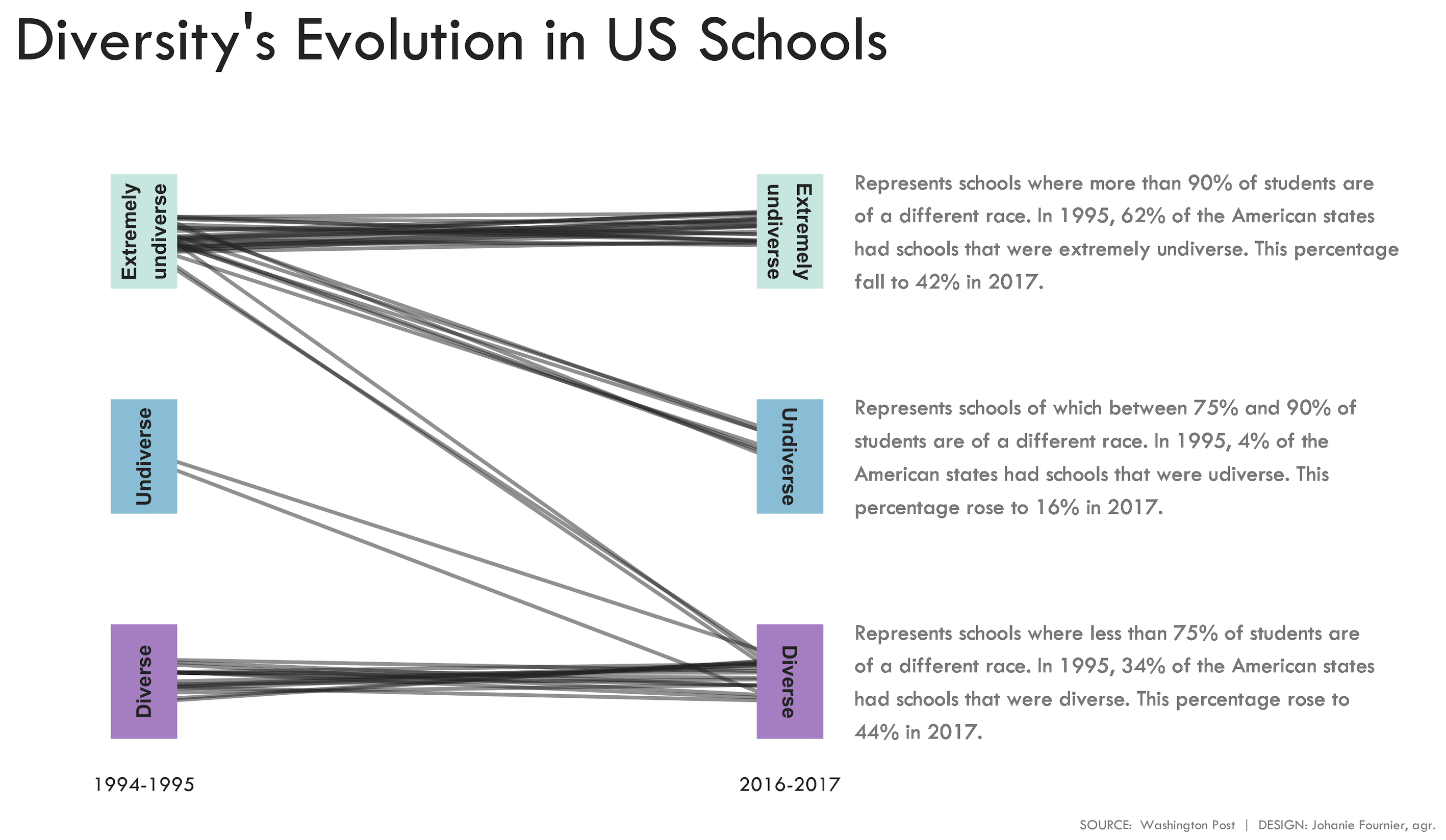
gg<-gg + labs(title="Diversity's Evolution in US Schools\n",
subtitle = " ",
x=" ",
y=" ",
caption="\nSOURCE: Washington Post | DESIGN: Johanie Fournier, agr.")
gg<-gg + theme( plot.title = element_text(size=37, hjust=0,vjust=0.5, family="Tw Cen MT", color="#2E2E2E"),
plot.subtitle = element_blank(),
plot.caption = element_text(size=8, hjust=1,vjust=0.5, family="Tw Cen MT", color="#8B8B8B"),
axis.title.y = element_blank(),
axis.title.x = element_blank(),
axis.text.x = element_text(size=12, hjust=0.5,vjust=0.5, family="Tw Cen MT", color="#2E2E2E"),
axis.text.y = element_blank())
#étiquette
gg <- gg + geom_text(aes(x = 2.1, y = 3),label = "Represents schools where more than 90% of students are\nof a different race. In 1995, 62% of the American states\nhad schools that were extremely undiverse. This percentage\nfall to 42% in 2017.", size = 4.5, family = "Tw Cen MT", color="#8B8B8B", hjust=0)
gg <- gg + geom_text(aes(x = 2.1, y = 2),label = "Represents schools of which between 75% and 90% of\nstudents are of a different race. In 1995, 4% of the\nAmerican states had schools that were udiverse. This\npercentage rose to 16% in 2017.", size = 4.5, family = "Tw Cen MT", color="#8B8B8B", hjust=0)
gg <- gg + geom_text(aes(x = 2.1, y = 1),label = "Represents schools where less than 75% of students are\nof a different race. In 1995, 34% of the American states\nhad schools that were diverse. This percentage rose to\n44% in 2017.", size = 4.5, family = "Tw Cen MT", color="#8B8B8B", hjust=0)
- Posted on:
- September 25, 2019
- Length:
- 4 minute read, 802 words
- Categories:
- rstats tidyverse tidytuesday
- Tags:
- rstats tidyverse tidytuesday