TyT2019W15 - Left_join or Right_join?

Get the data

player_dob <- readr::read_csv("https://raw.githubusercontent.com/rfordatascience/tidytuesday/master/data/2019/2019-04-09/player_dob.csv")

## Rows: 105 Columns: 5

## ── Column specification ────────────────────────────────────────────────────────
## Delimiter: ","
## chr  (2): name, grand_slam
## dbl  (1): age
## date (2): date_of_birth, date_of_first_title

## 
## ℹ Use `spec()` to retrieve the full column specification for this data.
## ℹ Specify the column types or set `show_col_types = FALSE` to quiet this message.

grand_slams <- readr::read_csv("https://raw.githubusercontent.com/rfordatascience/tidytuesday/master/data/2019/2019-04-09/grand_slams.csv")

## Rows: 416 Columns: 6

## ── Column specification ────────────────────────────────────────────────────────
## Delimiter: ","
## chr  (3): grand_slam, name, gender
## dbl  (2): year, rolling_win_count
## date (1): tournament_date

## 
## ℹ Use `spec()` to retrieve the full column specification for this data.
## ℹ Specify the column types or set `show_col_types = FALSE` to quiet this message.

grand_slam_timeline <- readr::read_csv("https://raw.githubusercontent.com/rfordatascience/tidytuesday/master/data/2019/2019-04-09/grand_slam_timeline.csv")

## Rows: 12605 Columns: 5

## ── Column specification ────────────────────────────────────────────────────────
## Delimiter: ","
## chr (4): player, tournament, outcome, gender
## dbl (1): year

## 
## ℹ Use `spec()` to retrieve the full column specification for this data.
## ℹ Specify the column types or set `show_col_types = FALSE` to quiet this message.

Explore the data

summary(player_dob)

##      name            grand_slam        date_of_birth       
##  Length:105         Length:105         Min.   :1934-11-02  
##  Class :character   Class :character   1st Qu.:1956-03-19  
##  Mode  :character   Mode  :character   Median :1971-08-12  
##                                        Mean   :1968-10-21  
##                                        3rd Qu.:1981-08-08  
##                                        Max.   :1997-10-16  
##                                                            
##  date_of_first_title       age       
##  Min.   :1968-06-08   Min.   : 5961  
##  1st Qu.:1978-06-16   1st Qu.: 7512  
##  Median :1994-10-15   Median : 8286  
##  Mean   :1992-10-28   Mean   : 8531  
##  3rd Qu.:2004-06-06   3rd Qu.: 9502  
##  Max.   :2018-09-08   Max.   :12724  
##  NA's   :3            NA's   :3

summary(grand_slams)

##       year       grand_slam            name           rolling_win_count
##  Min.   :1968   Length:416         Length:416         Min.   : 1.000   
##  1st Qu.:1980   Class :character   Class :character   1st Qu.: 1.000   
##  Median :1993   Mode  :character   Mode  :character   Median : 4.000   
##  Mean   :1993                                         Mean   : 5.507   
##  3rd Qu.:2006                                         3rd Qu.: 8.000   
##  Max.   :2019                                         Max.   :23.000   
##  tournament_date         gender         
##  Min.   :1968-01-10   Length:416        
##  1st Qu.:1979-12-10   Class :character  
##  Median :1993-03-26   Mode  :character  
##  Mean   :1993-04-09                     
##  3rd Qu.:2006-02-16                     
##  Max.   :2019-01-10

summary(grand_slam_timeline)

##     player               year       tournament          outcome         
##  Length:12605       Min.   :1968   Length:12605       Length:12605      
##  Class :character   1st Qu.:1981   Class :character   Class :character  
##  Mode  :character   Median :1993   Mode  :character   Mode  :character  
##                     Mean   :1993                                        
##                     3rd Qu.:2005                                        
##                     Max.   :2019                                        
##     gender         
##  Length:12605      
##  Class :character  
##  Mode  :character  
##                    
##                    
## 

Prepare the data

gender<-grand_slams%>% #J'ai besion de sélectionner seulement le genre
  select(name, gender)%>% 
  distinct()

data<-data_age%>%
  mutate(age_y=round(age/365, digits = 0))%>% #modifier l'age pour l'avoir en année
  mutate(tournament_date=date_of_first_title)%>% #avoir le même nom de colonne pour joindre les fichiers
  left_join(gender, by="name")%>%
  mutate(annee=year(date_of_first_title))%>%
  select("name", "gender", "age_y", "date_of_first_title")

Visualize the data

gg<-ggplot(data=data, aes(x=decennie, y=age_moy, group=gender, color=gender))
gg<-gg + geom_line(size=3)
gg<-gg + geom_point(size=6)
gg<- gg +scale_color_manual(values=c("#931328", "#3E7BBC"))
gg<-gg + geom_point(size=5, color="#FFFFFF")
#Ajouter les étiquettes de données
gg<-gg + geom_text(data=data, aes(x=decennie, y=age_moy, label=round(age_moy, digits=0)), size=2.75, vjust=0.5, family="Calibri")
gg<- gg +scale_color_manual(values=c("#931328", "#3E7BBC"))
#modifier la légende
gg<-gg + theme(legend.position="none")
#ajuster les étiquettes des axes
gg<-gg + scale_y_continuous(breaks=seq(15, 35, 5),limits = c(15, 35))
#modifier le thème
gg<-gg +theme(panel.border = element_blank(),
              panel.background = element_rect(fill = "#FFFFFF", colour = "#FFFFFF"),
              plot.background = element_rect(fill = "#FFFFFF", colour = "#FFFFFF"),
              panel.grid.major.x= element_line(linetype="dotted", size=0.5, color="#9F9F9F"),
              panel.grid.major.y= element_blank(),
              panel.grid.minor = element_blank(),
              axis.line.y = element_blank(),
              axis.line.x = element_line(linetype="solid", size=1, color="#9F9F9F"),
              axis.ticks.x = element_line(linetype="solid", size=1, color="#9F9F9F"),
              axis.ticks.y = element_blank())
#ajouter les titres
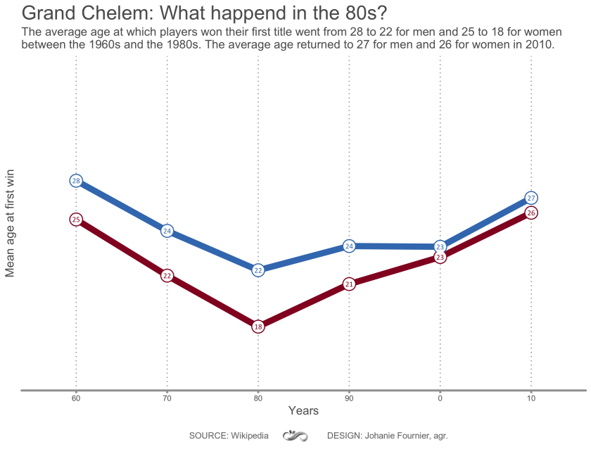
gg<-gg + labs(title= "Grand Chelem: What happend in the 80s?",
              subtitle="The average age at which players won their first title went from 28 to 22 for men and 25 to 18 for women\nbetween the 1960s and the 1980s. The average age returned to 27 for men and 26 for women in 2010.",
              y="Mean age at first win", 
              x="Years")
gg<-gg + theme(plot.title    = element_text(hjust=0,size=20, color="#5B5B5B"),
               plot.subtitle = element_text(hjust=0,size=12, color="#5B5B5B"),
               axis.title.x  = element_text(hjust=0.5, size=12,angle=360, color="#5B5B5B"),
               axis.title.y  = element_text(hjust=0.5, size=12, angle=90,color="#5B5B5B"),
               axis.text.y   = element_blank(), 
               axis.text.x   = element_text(hjust=0.5, size=8, color="#5B5B5B"))