TyT2019W11 - Side by Side
By Johanie Fournier, agr. in rstats tidyverse tidytuesday
March 12, 2019
Get the data
board_games <- readr::read_csv("https://raw.githubusercontent.com/rfordatascience/tidytuesday/master/data/2019/2019-03-12/board_games.csv")
## Rows: 10532 Columns: 22
## ── Column specification ────────────────────────────────────────────────────────
## Delimiter: ","
## chr (12): description, image, name, thumbnail, artist, category, compilation...
## dbl (10): game_id, max_players, max_playtime, min_age, min_players, min_play...
##
## ℹ Use `spec()` to retrieve the full column specification for this data.
## ℹ Specify the column types or set `show_col_types = FALSE` to quiet this message.
Explore the data
summary(board_games)
##     game_id       description           image            max_players
##  Min.   :     1   Length:10532       Length:10532       Min.   :  0.000
##  1st Qu.:  5444   Class :character   Class :character   1st Qu.:  4.000
##  Median : 28822   Mode  :character   Mode  :character   Median :  4.000
##  Mean   : 62059                                         Mean   :  5.657
##  3rd Qu.:126410                                         3rd Qu.:  6.000
##  Max.   :216725                                         Max.   :999.000
##   max_playtime         min_age        min_players     min_playtime
##  Min.   :    0.00   Min.   : 0.000   Min.   :0.000   Min.   :    0.00
##  1st Qu.:   30.00   1st Qu.: 8.000   1st Qu.:2.000   1st Qu.:   25.00
##  Median :   45.00   Median :10.000   Median :2.000   Median :   45.00
##  Mean   :   91.34   Mean   : 9.715   Mean   :2.071   Mean   :   80.88
##  3rd Qu.:   90.00   3rd Qu.:12.000   3rd Qu.:2.000   3rd Qu.:   90.00
##  Max.   :60000.00   Max.   :42.000   Max.   :9.000   Max.   :60000.00
##      name            playing_time       thumbnail         year_published
##  Length:10532       Min.   :    0.00   Length:10532       Min.   :1950
##  Class :character   1st Qu.:   30.00   Class :character   1st Qu.:1998
##  Mode  :character   Median :   45.00   Mode  :character   Median :2007
##                     Mean   :   91.34                      Mean   :2003
##                     3rd Qu.:   90.00                      3rd Qu.:2012
##                     Max.   :60000.00                      Max.   :2016
##     artist            category         compilation          designer
##  Length:10532       Length:10532       Length:10532       Length:10532
##  Class :character   Class :character   Class :character   Class :character
##  Mode  :character   Mode  :character   Mode  :character   Mode  :character
##
##
##
##   expansion            family            mechanic          publisher
##  Length:10532       Length:10532       Length:10532       Length:10532
##  Class :character   Class :character   Class :character   Class :character
##  Mode  :character   Mode  :character   Mode  :character   Mode  :character
##
##
##
##  average_rating   users_rated
##  Min.   :1.384   Min.   :   50.0
##  1st Qu.:5.830   1st Qu.:   85.0
##  Median :6.393   Median :  176.0
##  Mean   :6.371   Mean   :  870.1
##  3rd Qu.:6.943   3rd Qu.:  518.0
##  Max.   :9.004   Max.   :67655.0
Prepare the data
rate<-board_games%>%
  select(category,average_rating)%>% # conserver seulement les 2 colonnes pertinentes pour l'analyse
    mutate(category = str_replace_all(category, "\\/",","))%>% #uniformiser les séparateurs de catégories
    separate(category, c("no1","no2","no3","no4","no5","no6","no7","no8","no9","no10","no11","no12","no13","no14",
                         "no15"), sep=",")%>% #séparer les catégories en différents colonnes
  gather(key="No", value="Categories", -average_rating)%>%
  select(Categories,average_rating) %>%
  #summarise(mean=mean(average_rating)) # la note moyenne est de 6.37
  mutate(divergence=average_rating-6.37)%>%
  group_by(Categories)%>%
  summarise(average_div_rate=mean(divergence))

top_10<-rate%>%
  top_n(10, average_div_rate) #sélectionner les 10 meilleures évaluations

bottom_10<-rate%>%
  top_n(-10, average_div_rate)#sélectionner les 10 pires évaluations

rate<-top_10%>%
  rbind(bottom_10)
Visualize the data
#Graphique
gg<-ggplot(data=rate, aes(x=reorder(Categories, average_div_rate), y=average_div_rate, fill=Categories))
gg<-gg + geom_bar(stat="identity", width=0.85)
gg<-gg + coord_flip()
gg<-gg + scale_fill_manual(values = c("#A9A9A9", "#A9A9A9", "#A9A9A9", "#A9A9A9", "#A9A9A9", "#A9A9A9", "#A9A9A9", "#A9A9A9","#A9A9A9","#A9A9A9","#A9A9A9","#A9A9A9","#A9A9A9","#A9A9A9","#A9A9A9","#A9A9A9","#A9A9A9","#A44A3F","#090446","#A9A9A9"))
#Ajouter les étiquettes de données
gg<-gg + annotate(geom="text", x=1,y=-0.84, label="5.6", color="#A44A3F", size=4, hjust=0, fontface="bold")
gg<-gg + annotate(geom="text", x=20,y=0.85, label="7.2", color="#090446", size=4, hjust=0, fontface="bold")
gg<-gg + annotate(geom="text", x=1,y=0.02, label="Trivia", color="#A9A9A9", size=5, hjust=0)
gg<-gg + annotate(geom="text", x=2,y=0.02, label="Children's Game", color="#A9A9A9", size=5, hjust=0)
gg<-gg + annotate(geom="text", x=3,y=0.02, label="Memory", color="#A9A9A9", size=5, hjust=0)
gg<-gg + annotate(geom="text", x=4,y=0.02, label="Math", color="#A9A9A9", size=5, hjust=0)
gg<-gg + annotate(geom="text", x=5,y=0.02, label="Radio Theme", color="#A9A9A9", size=5, hjust=0)
gg<-gg + annotate(geom="text", x=6,y=0.02, label="TV", color="#A9A9A9", size=5, hjust=0)
gg<-gg + annotate(geom="text", x=7,y=0.02, label="Movies", color="#A9A9A9", size=5, hjust=0)
gg<-gg + annotate(geom="text", x=8,y=0.02, label="Electronic", color="#A9A9A9", size=5, hjust=0)
gg<-gg + annotate(geom="text", x=9,y=0.02, label="Music", color="#A9A9A9", size=5, hjust=0)
gg<-gg + annotate(geom="text", x=10,y=0.02, label="Word Game", color="#A9A9A9", size=5, hjust=0)
gg<-gg + annotate(geom="text", x=11,y=-0.02, label="Age of Reason", color="#A9A9A9", size=5, hjust=1)
gg<-gg + annotate(geom="text", x=12,y=-0.02, label="Post-Napoleonic", color="#A9A9A9", size=5, hjust=1)
gg<-gg + annotate(geom="text", x=13,y=-0.02, label="Miniature", color="#A9A9A9", size=5, hjust=1)
gg<-gg + annotate(geom="text", x=14,y=-0.02, label="Civilization", color="#A9A9A9", size=5, hjust=1)
gg<-gg + annotate(geom="text", x=15,y=-0.02, label="American Revolutionary War", color="#A9A9A9", size=5, hjust=1)
gg<-gg + annotate(geom="text", x=16,y=-0.02, label="American Indian Wars", color="#A9A9A9", size=5, hjust=1)
gg<-gg + annotate(geom="text", x=17,y=-0.02, label="Book", color="#A9A9A9", size=5, hjust=1)
gg<-gg + annotate(geom="text", x=18,y=-0.02, label="Civil War", color="#A9A9A9", size=5, hjust=1)
gg<-gg + annotate(geom="text", x=19,y=-0.02, label="Expansion for Base-game", color="#A9A9A9", size=5, hjust=1)
gg<-gg + annotate(geom="text", x=20,y=-0.02, label="Vietman War", color="#A9A9A9", size=5, hjust=1)
#modifier la légende
gg<-gg + theme(legend.position="none")
#modifier le thème
gg<-gg +theme(panel.border = element_blank(),
panel.background = element_rect(fill = "#FFFFFF", colour = "#FFFFFF"),
plot.background = element_rect(fill = "#FFFFFF", colour = "#FFFFFF"),
panel.grid.major.y= element_blank(),
panel.grid.major.x= element_blank(),
panel.grid.minor = element_blank(),
axis.line = element_blank(),
axis.ticks.y = element_blank(),
axis.ticks.x = element_blank())
#ajouter les titres
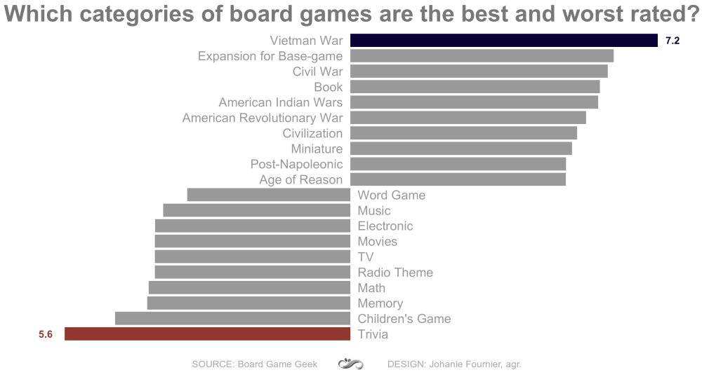
gg<-gg + labs(title="Which categories of board games are the best and worst rated?",
subtitle=NULL,
y=NULL,
x=NULL)
gg<-gg + theme(plot.title = element_text(hjust=0.5,size=26, color="#8B8B8B", face="bold"),
plot.subtitle = element_text(hjust=0,size=18, color="#8B8B8B"),
axis.title.y = element_blank(),
axis.title.x = element_blank(),
axis.text.y = element_blank(),
axis.text.x = element_blank())
- Posted on:
- March 12, 2019
- Length:
- 4 minute read, 724 words
- Categories:
- rstats tidyverse tidytuesday
- Tags:
- rstats tidyverse tidytuesday