TyT2019W48 - Put Together Two Histograms
By Johanie Fournier, agr. in rstats tidyverse tidytuesday
November 28, 2019
Get the data
loans <- readr::read_csv("https://raw.githubusercontent.com/rfordatascience/tidytuesday/master/data/2019/2019-11-26/loans.csv")
## Rows: 291 Columns: 10
## ── Column specification ────────────────────────────────────────────────────────
## Delimiter: ","
## chr (1): agency_name
## dbl (9): year, quarter, starting, added, total, consolidation, rehabilitatio...
##
## ℹ Use `spec()` to retrieve the full column specification for this data.
## ℹ Specify the column types or set `show_col_types = FALSE` to quiet this message.
Explore the data
summary(loans)
##  agency_name             year          quarter         starting
##  Length:291         Min.   :15.00   Min.   :1.000   Min.   :4.964e+07
##  Class :character   1st Qu.:16.00   1st Qu.:1.500   1st Qu.:9.311e+08
##  Mode  :character   Median :17.00   Median :2.000   Median :2.801e+09
##                     Mean   :16.74   Mean   :2.543   Mean   :3.878e+09
##                     3rd Qu.:17.00   3rd Qu.:4.000   3rd Qu.:6.615e+09
##                     Max.   :18.00   Max.   :4.000   Max.   :1.119e+10
##                                                     NA's   :9
##      added               total           consolidation      rehabilitation
##  Min.   :2.918e+08   Min.   :   212828   Min.   :   74574   Min.   :      -26
##  1st Qu.:5.430e+08   1st Qu.: 32888118   1st Qu.: 2977484   1st Qu.: 24843043
##  Median :9.127e+08   Median : 72669212   Median : 9508287   Median : 54501827
##  Mean   :1.305e+09   Mean   :106005716   Mean   :14950255   Mean   : 81592767
##  3rd Qu.:1.652e+09   3rd Qu.:167945568   3rd Qu.:23702274   3rd Qu.:123045718
##  Max.   :9.459e+09   Max.   :395249672   Max.   :52340470   Max.   :337310727
##  NA's   :160                                                NA's   :11
##  voluntary_payments wage_garnishments
##  Min.   :   19833   Min.   :     517
##  1st Qu.: 1270194   1st Qu.: 2527537
##  Median : 3464174   Median : 6317306
##  Mean   : 4590299   Mean   : 7956659
##  3rd Qu.: 8019843   3rd Qu.:11321348
##  Max.   :14687278   Max.   :28107801
##
Prepare the data
data <- loans %>%
  group_by(year, quarter) %>%
  summarise(dette=sum(starting, na.rm=TRUE),
            remboursement=sum(total, na.rm=TRUE)) %>%
  mutate(pourcentage=(remboursement/dette),
         aug_dette=(dette/113325957209)) %>%
  ungroup() %>%
  add_column(cent=20) %>%
  unite(annee, "cent", "year", sep="") %>%
  unite(date, annee, quarter, sep="-")
## `summarise()` has grouped output by 'year'. You can override using the `.groups` argument.
Visualize the data
gg<- ggplot(data=data,aes(x = date, y=aug_dette, group=1))
gg <- gg + geom_bar(stat="identity", width = 0.75, fill="#C8C8C8")
gg <- gg + geom_bar(aes(x=date, y=pourcentage),stat="identity", width = 0.60, fill="#FB5012")
#retirer la légende
gg <- gg + theme(legend.position = "none")
#ajuster les axes
gg<-gg + scale_y_continuous(breaks=seq(0,1,0.20), limits=c(0, 1), labels=scales::percent)
#ajouter les étiquettes
gg<-gg + geom_text(data=data, aes(x=date, y=pourcentage, label=paste0(round(data$pourcentage*100,1),"%", sep="")),
color="#FB5012", size=3, position = position_stack(vjust = 2.5), fontface="bold")
#retourner le graphique
gg<-gg + coord_flip()
#modifier le thème
gg <- gg + theme(panel.border = element_blank(),
panel.background = element_blank(),
plot.background = element_blank(),
panel.grid.major.x= element_line(size=0.5, color = "#C8C8C8", linetype = "dotted"),
panel.grid.major.y= element_blank(),
panel.grid.minor = element_blank(),
axis.line.x = element_blank(),
axis.line.y =element_blank(),
axis.ticks.x = element_blank(),
axis.ticks.y = element_blank())
#ajouter les titres
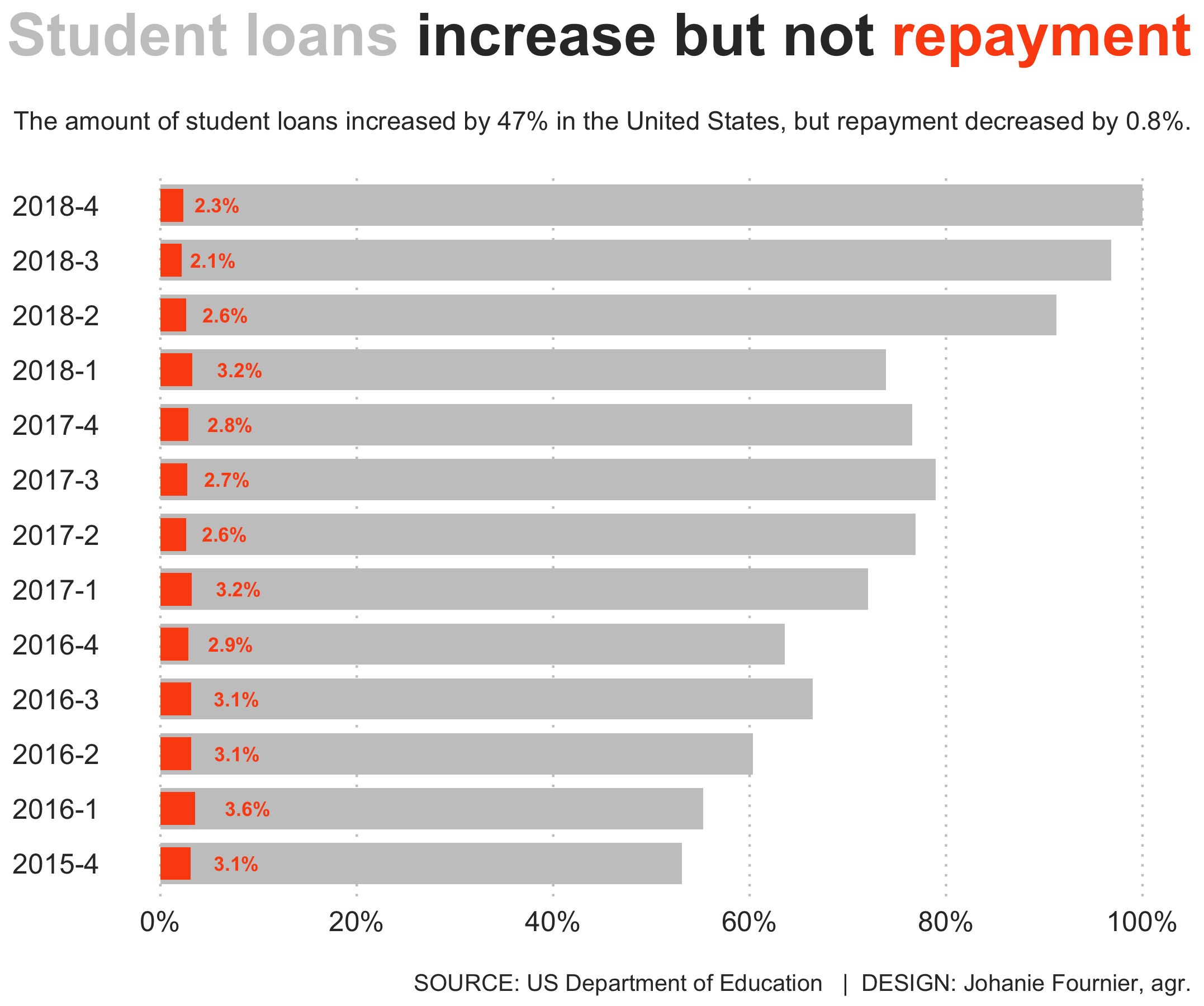
gg<-gg + labs(title="<span style='color:#C8C8C8'>**Student loans**</span> increase but not <span style='color:#FB5012'>**repayment**</span>",
subtitle = "\nThe amount of student loans increased by 47% in the United States, but repayment decreased by 0.8%.\n",
x=" ",
y=" ",
caption="\nSOURCE: US Department of Education | DESIGN: Johanie Fournier, agr.")
gg<-gg + theme( plot.title = element_markdown(lineheight = 1.1,size=25.5, hjust=1,vjust=0.5, face="bold", color="#333333"),
plot.subtitle = element_text(size=11, hjust=1,vjust=0.5, color="#333333"),
plot.caption = element_text(size=10, hjust=1,vjust=0.5, color="#333333"),
axis.title.y = element_blank(),
axis.title.x = element_blank(),
axis.text.y = element_text(size=12, hjust=0,vjust=0.5, color="#333333"),
axis.text.x = element_text(size=12, hjust=0.5,vjust=0.5, color="#333333"))
- Posted on:
- November 28, 2019
- Length:
- 3 minute read, 477 words
- Categories:
- rstats tidyverse tidytuesday
- Tags:
- rstats tidyverse tidytuesday