TyT2019W49 - Visualize Mean Price

By Johanie Fournier, agr. in rstats tidyverse tidytuesday

December 7, 2019

Get the data

tickets <- readr::read_csv("https://raw.githubusercontent.com/rfordatascience/tidytuesday/master/data/2019/2019-12-03/tickets.csv")

## Rows: 1260891 Columns: 7

## ── Column specification ────────────────────────────────────────────────────────
## Delimiter: ","
## chr  (2): violation_desc, issuing_agency
## dbl  (4): fine, lat, lon, zip_code
## dttm (1): issue_datetime

## 
## ℹ Use `spec()` to retrieve the full column specification for this data.
## ℹ Specify the column types or set `show_col_types = FALSE` to quiet this message.

Explore the data

summary(tickets)

##  violation_desc     issue_datetime                     fine        
##  Length:1260891     Min.   :2017-01-01 00:00:00   Min.   :  15.00  
##  Class :character   1st Qu.:2017-04-05 00:37:30   1st Qu.:  26.00  
##  Mode  :character   Median :2017-07-05 09:11:00   Median :  36.00  
##                     Mean   :2017-07-03 06:07:59   Mean   :  45.41  
##                     3rd Qu.:2017-10-01 13:20:30   3rd Qu.:  51.00  
##                     Max.   :2017-12-31 15:42:00   Max.   :1001.00  
##                                                                    
##  issuing_agency          lat             lon            zip_code     
##  Length:1260891     Min.   :39.57   Min.   :-75.99   Min.   :19102   
##  Class :character   1st Qu.:39.95   1st Qu.:-75.18   1st Qu.:19106   
##  Mode  :character   Median :39.95   Median :-75.16   Median :19123   
##                     Mean   :39.97   Mean   :-75.16   Mean   :19124   
##                     3rd Qu.:39.97   3rd Qu.:-75.15   3rd Qu.:19143   
##                     Max.   :40.37   Max.   :-74.96   Max.   :19154   
##                                                      NA's   :173588

glimpse(tickets)

## Rows: 1,260,891
## Columns: 7
## $ violation_desc <chr> "BUS ONLY ZONE", "STOPPING PROHIBITED", "OVER TIME LIMI…
## $ issue_datetime <dttm> 2017-12-06 12:29:00, 2017-10-16 18:03:00, 2017-11-02 2…
## $ fine           <dbl> 51, 51, 26, 26, 76, 51, 36, 36, 76, 26, 26, 301, 36, 51…
## $ issuing_agency <chr> "PPA", "PPA", "PPA", "PPA", "PPA", "POLICE", "PPA", "PP…
## $ lat            <dbl> 40.03550, 40.02571, 40.02579, 40.02590, 39.95617, 40.03…
## $ lon            <dbl> -75.08111, -75.22249, -75.22256, -75.22271, -75.16603, …
## $ zip_code       <dbl> 19149, 19127, 19127, 19127, 19102, NA, NA, 19106, 19147…

Prepare the data

issuing_agency<-tickets %>%
     select('issuing_agency') %>%
     inspect_cat()

data<-tickets %>% 
  mutate(date=as.Date(floor_date(issue_datetime,"month"))) %>% 
  group_by(issuing_agency, date) %>% 
  summarise(total=sum(fine), count=n()) %>% 
  mutate(moyenne=total/count)

## `summarise()` has grouped output by 'issuing_agency'. You can override using the `.groups` argument.

data_housing<-data %>% 
  filter(issuing_agency=="HOUSING")

Visualize the data

gg<- ggplot(data=data,aes(x = date, y=moyenne, group=issuing_agency))
gg <- gg +  geom_line(color="#C0C0C0", size=1.3)
gg <- gg +  geom_line(data=data_housing,aes(x = date, y=moyenne, group=issuing_agency), color="#89023E", size=1.3)
#ajuster les axes
gg <- gg +  scale_x_date(labels = date_format("%B"), date_breaks = "1 months")
gg <- gg +  scale_y_continuous(breaks=seq(0,130,20), limits=c(0, 130), expand=c(0.01,0))
#retirer la légende
gg <- gg +  theme(legend.position = "none")
#modifier le thème
gg <- gg +  theme(  panel.border = element_rect(color="#333333", ,size=1, fill=NA),
                    panel.background = element_rect(fill ="#333333"),
                    plot.background = element_rect(fill="#333333"),
                    panel.grid.major.y= element_line(size=0.5, color = "#616161", linetype = "dotted"),
                    panel.grid.major.x= element_blank(),
                    panel.grid.minor = element_blank(),
                    axis.line.x = element_blank(),
                    axis.line.y =element_blank(),
                    axis.ticks.x = element_blank(), 
                    axis.ticks.y = element_blank())
#ajouter les titres
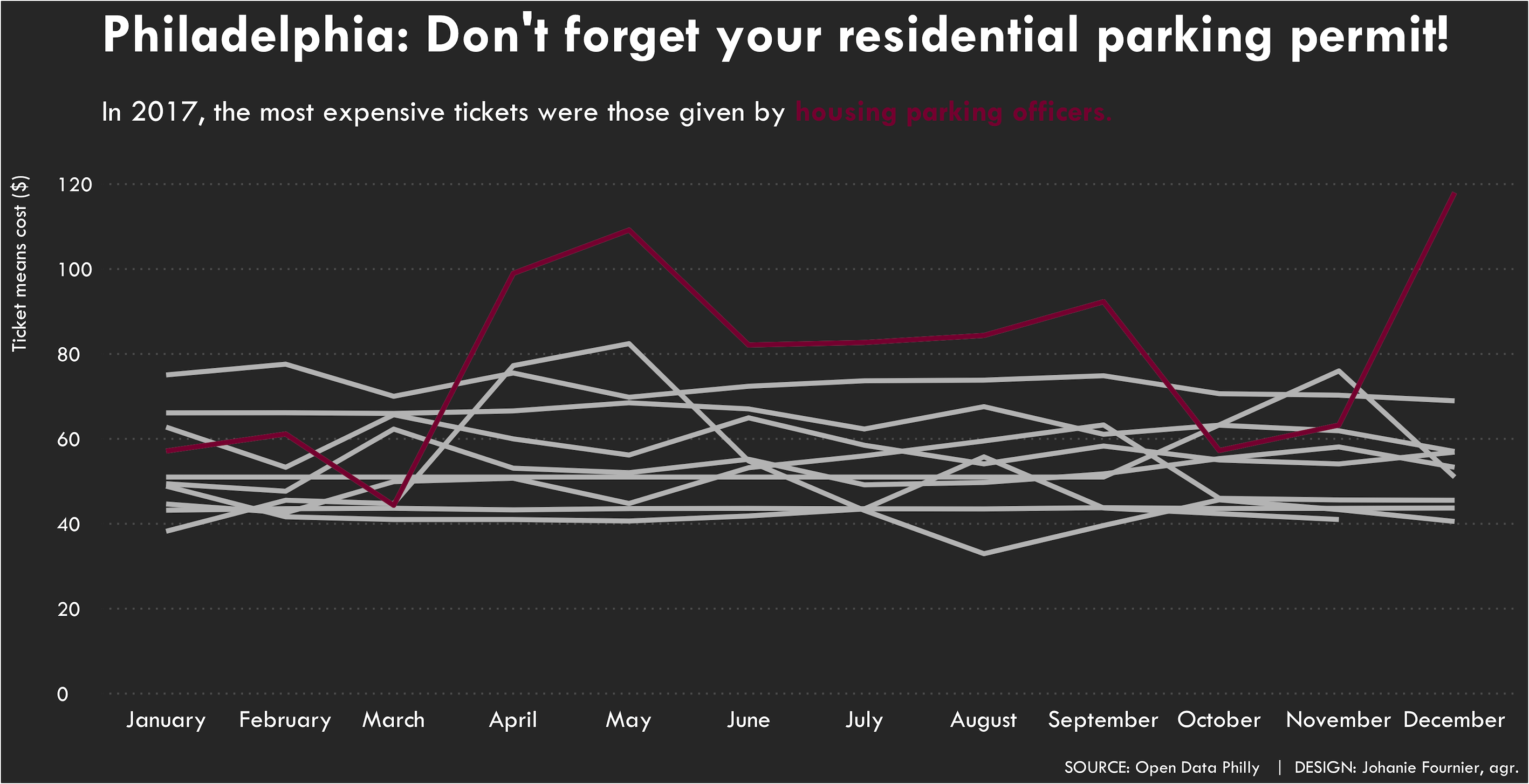
gg<-gg + labs(title="Philadelphia: Don't forget your residential parking permit!",
              subtitle = "<br>In 2017, the most expensive tickets were those given by <span style='color:#89023E'>**housing parking officers**.</span>",
              x=" ", 
              y="Ticket means cost ($)\n", 
              caption="\nSOURCE: Open Data Philly   |  DESIGN: Johanie Fournier, agr.")
gg<-gg + theme(  plot.title    =  element_text(size=31, hjust=0,vjust=0.5, color="#FFFFFF", family="Tw Cen MT", face="bold"),
                 plot.subtitle = element_markdown(lineheight = 1.1,size=17, hjust=0,vjust=0.5, color="#FFFFFF", family="Tw Cen MT"),
                 plot.caption  = element_text(size=10, hjust=1,vjust=0.5, color="#FFFFFF", family="Tw Cen MT"),
                 axis.title.y  = element_text(size=12, hjust=0.9,vjust=0.5, color="#FFFFFF", family="Tw Cen MT", angle=90),
                 axis.title.x  = element_blank(),
                 axis.text.y   = element_text(size=12, hjust=0,vjust=0.5, color="#FFFFFF", family="Tw Cen MT"), 
                 axis.text.x   = element_text(size=14, hjust=0.5,vjust=0.5, color="#FFFFFF", family="Tw Cen MT"))

Posted on:: December 7, 2019

Length:: 3 minute read, 505 words

Categories:: rstats tidyverse tidytuesday

Tags:: rstats tidyverse tidytuesday

See Also:: Predicting MO with H2O Models from IRDA data; IRDA soil data; This is the begining of a cheat sheet!