TyT2020W03 - Percentage by Category
By Johanie Fournier, agr. in rstats tidyverse tidytuesday
January 15, 2020
Get the data
passwords <- readr::read_csv('https://raw.githubusercontent.com/rfordatascience/tidytuesday/master/data/2020/2020-01-14/passwords.csv')
## Rows: 507 Columns: 9
## ── Column specification ────────────────────────────────────────────────────────
## Delimiter: ","
## chr (3): password, category, time_unit
## dbl (6): rank, value, offline_crack_sec, rank_alt, strength, font_size
##
## ℹ Use `spec()` to retrieve the full column specification for this data.
## ℹ Specify the column types or set `show_col_types = FALSE` to quiet this message.
Explore the data
summary(passwords)
##       rank         password           category             value
##  Min.   :  1.0   Length:507         Length:507         Min.   : 1.290
##  1st Qu.:125.8   Class :character   Class :character   1st Qu.: 3.430
##  Median :250.5   Mode  :character   Mode  :character   Median : 3.720
##  Mean   :250.5                                         Mean   : 5.603
##  3rd Qu.:375.2                                         3rd Qu.: 3.720
##  Max.   :500.0                                         Max.   :92.270
##  NA's   :7                                             NA's   :7
##   time_unit         offline_crack_sec     rank_alt        strength
##  Length:507         Min.   : 0.00000   Min.   :  1.0   Min.   : 0.000
##  Class :character   1st Qu.: 0.00321   1st Qu.:125.8   1st Qu.: 6.000
##  Mode  :character   Median : 0.00321   Median :251.5   Median : 7.000
##                     Mean   : 0.50001   Mean   :251.2   Mean   : 7.432
##                     3rd Qu.: 0.08350   3rd Qu.:376.2   3rd Qu.: 8.000
##                     Max.   :29.27000   Max.   :502.0   Max.   :48.000
##                     NA's   :7          NA's   :7       NA's   :7
##    font_size
##  Min.   : 0.0
##  1st Qu.:10.0
##  Median :11.0
##  Mean   :10.3
##  3rd Qu.:11.0
##  Max.   :28.0
##  NA's   :7
glimpse(passwords)
## Rows: 507
## Columns: 9
## $ rank              <dbl> 1, 2, 3, 4, 5, 6, 7, 8, 9, 10, 11, 12, 13, 14, 15, 1…
## $ password          <chr> "password", "123456", "12345678", "1234", "qwerty", …
## $ category          <chr> "password-related", "simple-alphanumeric", "simple-a…
## $ value             <dbl> 6.91, 18.52, 1.29, 11.11, 3.72, 1.85, 3.72, 6.91, 6.…
## $ time_unit         <chr> "years", "minutes", "days", "seconds", "days", "minu…
## $ offline_crack_sec <dbl> 2.170e+00, 1.110e-05, 1.110e-03, 1.110e-07, 3.210e-0…
## $ rank_alt          <dbl> 1, 2, 3, 4, 5, 6, 7, 8, 9, 10, 11, 12, 13, 14, 15, 1…
## $ strength          <dbl> 8, 4, 4, 4, 8, 4, 8, 4, 7, 8, 8, 1, 32, 9, 9, 8, 8, …
## $ font_size         <dbl> 11, 8, 8, 8, 11, 8, 11, 8, 11, 11, 11, 4, 23, 12, 12…
Prepare the data
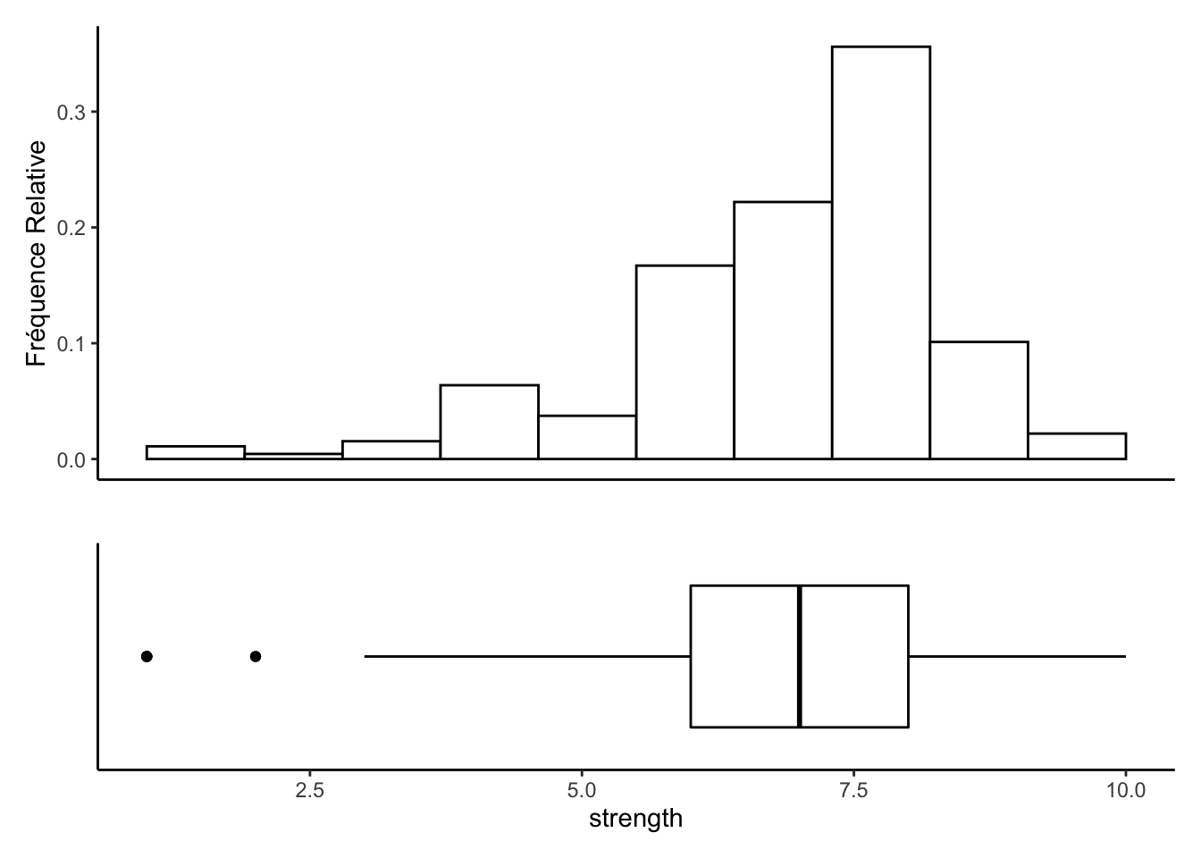
plt1 <-passwords %>%
  filter(strength<=10& strength>=1) %>%
  ggplot(aes(x=" ", y = strength)) +
  geom_boxplot(fill = "#FFFFFF", color = "black") +
  coord_flip() +
  theme_classic() +
  xlab("") +
  ylab("strength")+
  theme(axis.text.y=element_blank(),
        axis.ticks.y=element_blank())

plt2 <-passwords %>%
  filter(strength<=10 & strength>=1) %>%
  ggplot() +
   geom_histogram(aes(x = strength, y = (..count..)/sum(..count..)),
                       position = "identity", binwidth = 1,
                       fill = "#FFFFFF", color = "black") +
   ylab("Fréquence Relative")+
   xlab("")+
  theme_classic()+
  theme(axis.text.x = element_blank())+
  theme(axis.ticks.x = element_blank())
plt2 + plt1 + plot_layout(nrow = 2, heights = c(2, 1))
data<-passwords %>%
  filter(strength<=10 & strength>=1)

summary(data)
##       rank         password           category             value
##  Min.   :  1.0   Length:455         Length:455         Min.   : 1.290
##  1st Qu.:122.5   Class :character   Class :character   1st Qu.: 3.430
##  Median :244.0   Mode  :character   Mode  :character   Median : 3.720
##  Mean   :247.7                                         Mean   : 4.594
##  3rd Qu.:374.0                                         3rd Qu.: 3.720
##  Max.   :499.0                                         Max.   :18.520
##   time_unit         offline_crack_sec      rank_alt        strength
##  Length:455         Min.   :0.0000001   Min.   :  1.0   Min.   : 1.000
##  Class :character   1st Qu.:0.0032100   1st Qu.:122.5   1st Qu.: 6.000
##  Mode  :character   Median :0.0032100   Median :245.0   Median : 7.000
##                     Mean   :0.2799016   Mean   :248.4   Mean   : 7.042
##                     3rd Qu.:0.0835000   3rd Qu.:375.0   3rd Qu.: 8.000
##                     Max.   :2.1700000   Max.   :501.0   Max.   :10.000
##    font_size
##  Min.   : 4.00
##  1st Qu.:10.00
##  Median :11.00
##  Mean   :10.55
##  3rd Qu.:11.00
##  Max.   :13.00
data<-passwords %>%
  filter(strength<=10 & strength>=1) %>%
       mutate(force=case_when(strength >= 8 ~ "fort",
                             strength <= 6 ~ "mauvais",
                             strength >6 & strength<8 ~ "moyen")) %>%
  count(category, force) %>%
  spread(force, n) %>%
  mutate(Fort=fort/(fort+moyen+mauvais)*100) %>%
  mutate(Moyen=moyen/(fort+moyen+mauvais)*100) %>%
  mutate(Mauvais=mauvais/(fort+moyen+mauvais)*100) %>%
  filter(!category=="food")
Visualize the data
#Graphique
gg<- ggplot(data=data,aes(x = pct_fort, y=reorder(category, pct_fort), group=category))
gg <- gg + geom_point(color="#ffffff",fill="#F7B32B", size=17, pch=21)
gg <- gg + geom_segment( aes(x=0, xend=100,y=category, yend=category),
color="#838A90", alpha=0.6, size=4)
gg <- gg + geom_segment( aes(x=0, xend=100,y=category, yend=category),
color="#ffffff", alpha=1, size=0.5)
gg <- gg + geom_point(color="#ffffff",fill="#F7B32B", size=18, pch=21)
#ajouter les étiquettes de points
gg<-gg + geom_text(data=data, aes(x=pct_fort, y=category, label=(paste0(round(data$pct_fort,0),"%")), group=NULL), color="#ffffff", size=4.5, vjust=0.5, hjust=0.5, fontface="bold")
#modifier le thème
gg <- gg + theme(plot.background = element_rect(fill = "#173f50"),
panel.background = element_rect(fill = "#173f50"),
panel.grid.major.y= element_blank(),
panel.grid.major.x= element_blank(),
panel.grid.minor = element_blank(),
axis.line.x = element_blank(),
axis.line.y =element_blank(),
axis.ticks.x = element_blank(),
axis.ticks.y = element_blank())
#ajouter les titres
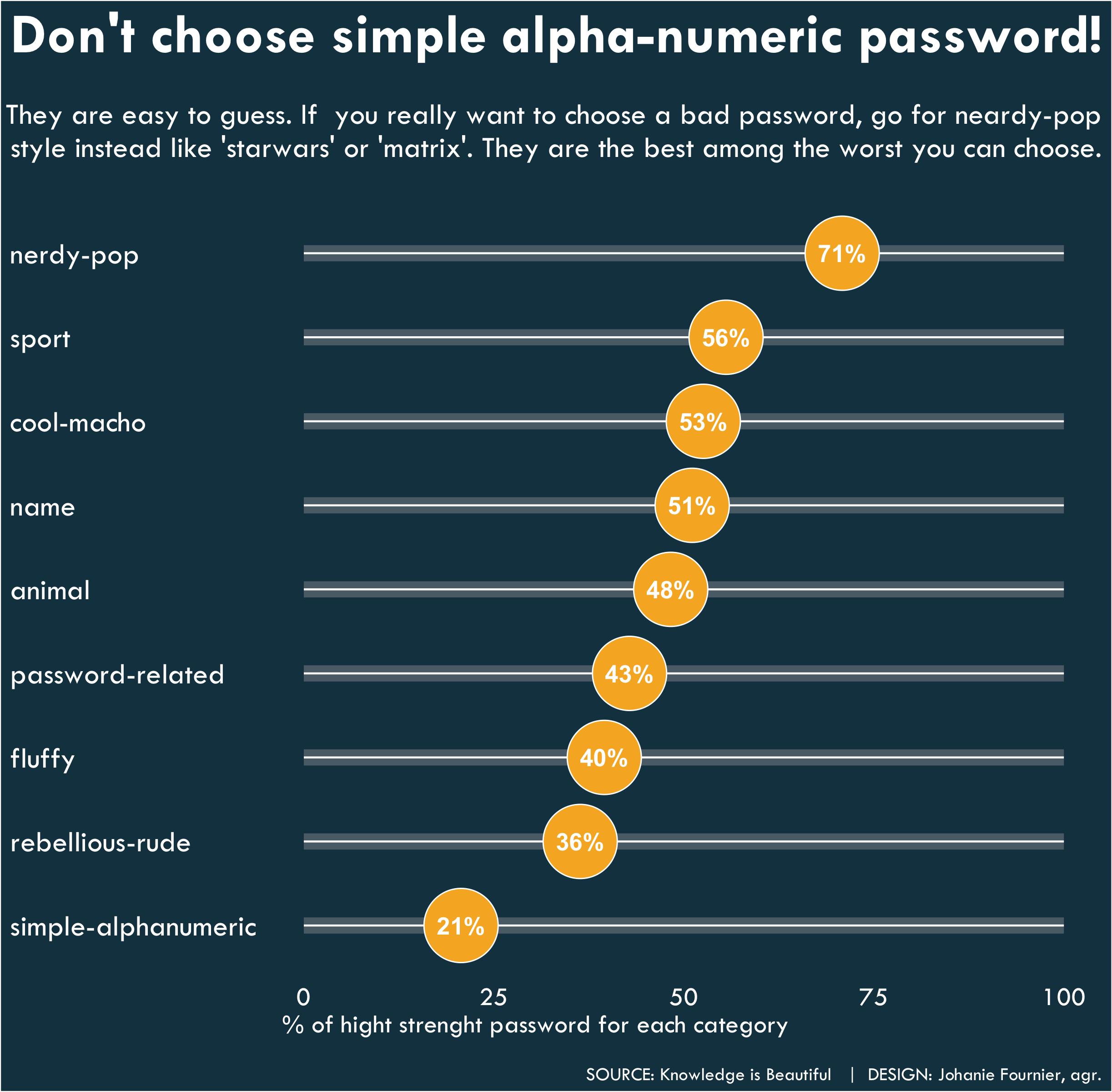
gg<-gg + labs(title="Don't choose simple alpha-numeric password!",
subtitle = "\nThey are easy to guess. If you really want to choose a bad password, go for neardy-pop\nstyle instead like 'starwars' or 'matrix'. They are the best among the worst you can choose.\n",
x="% of hight strenght password for each category",
y=" ",
caption="\nSOURCE: Knowledge is Beautiful | DESIGN: Johanie Fournier, agr.")
gg<-gg + theme( plot.title = element_text(size=30, hjust=1,vjust=0.5, color="#FFFFFF", family="Tw Cen MT", face="bold"),
plot.subtitle = element_text(size=16.1, hjust=1,vjust=0.5, color="#FFFFFF", family="Tw Cen MT"),
plot.caption = element_text(size=10, hjust=1,vjust=0.5, color="#FFFFFF", family="Tw Cen MT"),
axis.title.x = element_text(size=14, hjust=0.05,vjust=0.5, color="#FFFFFF", family="Tw Cen MT", angle =0),
axis.title.y = element_blank(),
axis.text.y = element_text(size=16, hjust=0,vjust=0.5, color="#FFFFFF", family="Tw Cen MT"),
axis.text.x = element_text(size=14, hjust=0.5,vjust=0.5, color="#FFFFFF", family="Tw Cen MT"))
- Posted on:
- January 15, 2020
- Length:
- 4 minute read, 825 words
- Categories:
- rstats tidyverse tidytuesday
- Tags:
- rstats tidyverse tidytuesday