TyT2020W06 - Facet Wrap and Areas Under the Curve
By Johanie Fournier, agr. in rstats tidyverse tidytuesday
February 8, 2020
Get the data
attendance <- readr::read_csv("https://raw.githubusercontent.com/rfordatascience/tidytuesday/master/data/2020/2020-02-04/attendance.csv")
## Rows: 10846 Columns: 8
## ── Column specification ────────────────────────────────────────────────────────
## Delimiter: ","
## chr (2): team, team_name
## dbl (6): year, total, home, away, week, weekly_attendance
##
## ℹ Use `spec()` to retrieve the full column specification for this data.
## ℹ Specify the column types or set `show_col_types = FALSE` to quiet this message.
Explore the data
summary(attendance)
##      team            team_name              year          total
##  Length:10846       Length:10846       Min.   :2000   Min.   : 760644
##  Class :character   Class :character   1st Qu.:2005   1st Qu.:1040509
##  Mode  :character   Mode  :character   Median :2010   Median :1081090
##                                        Mean   :2010   Mean   :1080910
##                                        3rd Qu.:2015   3rd Qu.:1123230
##                                        Max.   :2019   Max.   :1322087
##
##       home             away             week    weekly_attendance
##  Min.   :202687   Min.   :450295   Min.   : 1   Min.   : 23127
##  1st Qu.:504360   1st Qu.:524974   1st Qu.: 5   1st Qu.: 63246
##  Median :543185   Median :541757   Median : 9   Median : 68334
##  Mean   :540455   Mean   :540455   Mean   : 9   Mean   : 67557
##  3rd Qu.:578342   3rd Qu.:557741   3rd Qu.:13   3rd Qu.: 72545
##  Max.   :741775   Max.   :601655   Max.   :17   Max.   :105121
##                                                 NA's   :638
glimpse(attendance)
## Rows: 10,846
## Columns: 8
## $ team              <chr> "Arizona", "Arizona", "Arizona", "Arizona", "Arizona…
## $ team_name         <chr> "Cardinals", "Cardinals", "Cardinals", "Cardinals", …
## $ year              <dbl> 2000, 2000, 2000, 2000, 2000, 2000, 2000, 2000, 2000…
## $ total             <dbl> 893926, 893926, 893926, 893926, 893926, 893926, 8939…
## $ home              <dbl> 387475, 387475, 387475, 387475, 387475, 387475, 3874…
## $ away              <dbl> 506451, 506451, 506451, 506451, 506451, 506451, 5064…
## $ week              <dbl> 1, 2, 3, 4, 5, 6, 7, 8, 9, 10, 11, 12, 13, 14, 15, 1…
## $ weekly_attendance <dbl> 77434, 66009, NA, 71801, 66985, 44296, 38293, 62981,…
Prepare the data
data<-attendance %>%
  select(team, team_name, year, total,home, away) %>%
  distinct() %>%
  mutate(pct_home=(home/total*100)-50) %>%
  select(team_name, year, pct_home)
Visualize the data
#Graphique
gg<- ggplot(data=data,aes(x = year, y=pct_home, group=team_name))
gg<-gg + geom_line(size=1, color="white")
gg<-gg + geom_ribbon(aes(x=year,ymax=pct_home,fill="#731963"),ymin=0,alpha=0.3)
#gg<-gg + geom_ribbon(aes(x=year,ymin=pct_home,fill="#F0E100"),ymax=100,,alpha=0.3)
gg<-gg + facet_wrap(.~team_name)
#ajuster la légende
gg<-gg + theme(legend.position = "null")
#ajuster les axes
gg<-gg + scale_y_continuous(breaks=seq(-10, 10, 5), limits = c(-10,10))
gg<-gg + scale_x_continuous(breaks=seq(2000, 2019, 19), limits = c(2000,2019))
#modifier le thème
gg <- gg + theme(plot.background = element_rect(fill = "#171717"),
panel.background = element_rect(fill = "#171717"),
panel.grid.major.y= element_blank(),
panel.grid.major.x= element_blank(),
panel.grid.minor = element_blank(),
axis.line.x = element_line(color="white"),
axis.line.y = element_line(color="white"),
axis.ticks.x = element_blank(),
axis.ticks.y = element_blank())
#ajuster le facet_wrap
gg<-gg + theme(strip.background = element_blank(),
strip.text.x = element_text(color="white", size=16, hjust=0))
#ajouter les titres
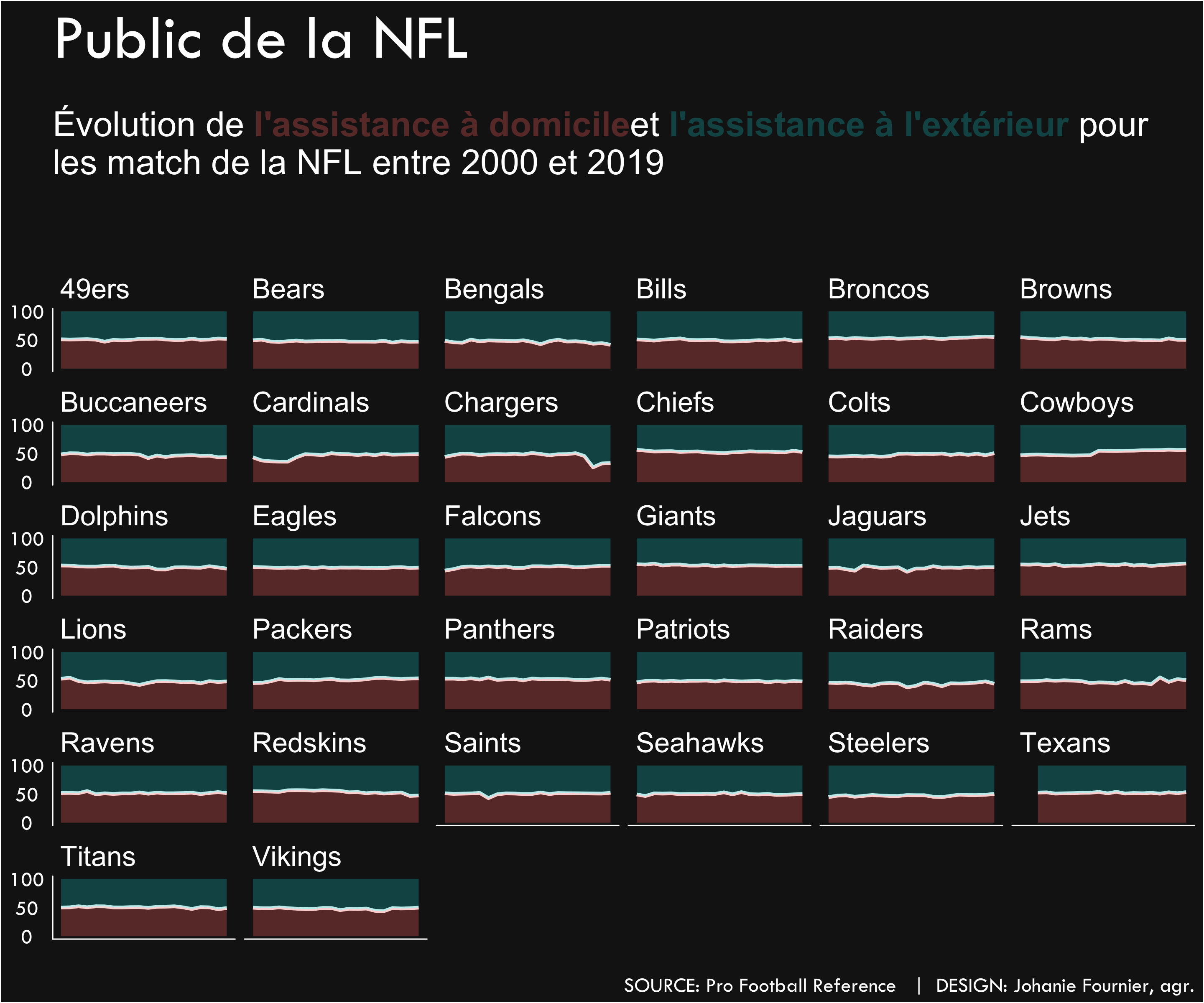
gg<-gg + labs(title="Public de la NFL",
subtitle = "<br>Évolution de <span style='color:#6A3734'>**l'assistance à domicile**</span> pour les match de la NFL entre<br>2000 et 2019<br><br>",
#et <span style='color:#155355'>**l'assistance à l'extérieur**</span> pour<br>
x=" ",
y="Déviation de 50%",
caption="\nSOURCE: Pro Football Reference | DESIGN: Johanie Fournier, agr.")
gg<-gg + theme( plot.title = element_text(size=37, hjust=0,vjust=0.5, family="Tw Cen MT", color="white"),
plot.subtitle = element_markdown(lineheight = 1.1,size=20, hjust=0,vjust=0.5, color="white"),
plot.caption = element_text(size=12, hjust=1,vjust=0.5, family="Tw Cen MT", color="white"),
axis.title.y = element_text(size=14, hjust=1,vjust=0.5, family="Tw Cen MT", color="white"),
axis.title.x = element_blank(),
axis.text.x = element_blank(),
axis.text.y = element_text(size=12, hjust=0.5,vjust=0.5, family="Tw Cen MT", color="white"))
- Posted on:
- February 8, 2020
- Length:
- 3 minute read, 498 words
- Categories:
- rstats tidyverse tidytuesday
- Tags:
- rstats tidyverse tidytuesday