TyT2019W28 - Sankey Diagram

wwc_outcomes <- readr::read_csv("https://raw.githubusercontent.com/rfordatascience/tidytuesday/master/data/2019/2019-07-09/wwc_outcomes.csv")

codes <- readr::read_csv("https://raw.githubusercontent.com/rfordatascience/tidytuesday/master/data/2019/2019-07-09/codes.csv")

summary(wwc_outcomes)

summary(codes)

data<-wwc_outcomes%>%
  left_join(codes, by = "team") %>% 
  mutate(country=ifelse(country=="Brazil", "Brésil", country)) %>% 
  mutate(country=ifelse(country=="Germany", "Allemagne", country)) %>% 
  mutate(country=ifelse(country=="Japan", "Japon", country)) %>% 
  mutate(country=ifelse(country=="Norway", "Norvège", country)) %>% 
  mutate(country=ifelse(country=="Sweden", "Suède", country)) %>% 
  mutate(country=ifelse(country=="United States", "États-Unis", country)) %>% 
  mutate(country=ifelse(country=="North Korea", "Corée du Nord", country)) %>% 
  mutate(country=ifelse(country=="England", "Angleterre", country)) %>%
  arrange(year,yearly_game_id, team_num) %>% 
  mutate(equipe_gagante=country) %>% 
  mutate(equipe_perdante=lead(country)) %>% 
  filter(!is.na(equipe_perdante)) %>% 
  select(equipe_gagante, equipe_perdante) %>% 
  group_by(equipe_gagante, equipe_perdante) %>% 
  summarise(freq=n()) %>% 
  filter(freq>4) %>% 
  ungroup() %>%
  mutate(equipe_gagante = factor(equipe_gagante,
                        levels = c("Brésil", "Canada", "Allemagne",
                                   "Japon", "Norvège", "Suède",
                                   "États-Unis")))

#Graphique 
data<-wwc_outcomes%>%
  left_join(codes, by = "team") %>% 
  arrange(year,yearly_game_id, team_num) %>% 
  mutate(equipe_gagante=country) %>% 
  mutate(equipe_perdante=lead(country)) %>% 
  filter(!is.na(equipe_perdante)) %>% 
  select(equipe_gagante, equipe_perdante) %>% 
  group_by(equipe_gagante, equipe_perdante) %>% 
  summarise(freq=n()) %>% 
  filter(freq>4) 

gg<-ggplot(data=data, aes(axis1 = equipe_gagante, axis2 = equipe_perdante, y=freq))
gg<-gg + geom_alluvium(aes(fill = equipe_gagante), width = 1/7)
gg<-gg + geom_stratum(width = 1/7, alpha=0.5, color = "black") 
gg<-gg + geom_text(stat = "stratum", label.strata = TRUE) 
gg<-gg + scale_fill_manual(values = c("#736F6E", "#736F6E", "#018E42","#736F6E", "#736F6E", "#736F6E", "#736F6E"))
#ajuster les axes 
gg<-gg + scale_x_discrete(limits = c("Winning Team", "Losing Team"), expand = c(.05, .05), position = "top")
#modifier la légende
gg<-gg + theme(legend.position="none")
#modifier le thème
gg<-gg +theme(panel.border = element_blank(),
              panel.background = element_blank(),
              plot.background = element_blank(),
              panel.grid.major.y= element_blank(),
              panel.grid.major.x= element_blank(),
              panel.grid.minor = element_blank(),
              axis.line = element_blank(),
              axis.ticks= element_blank())
#ajouter les titres
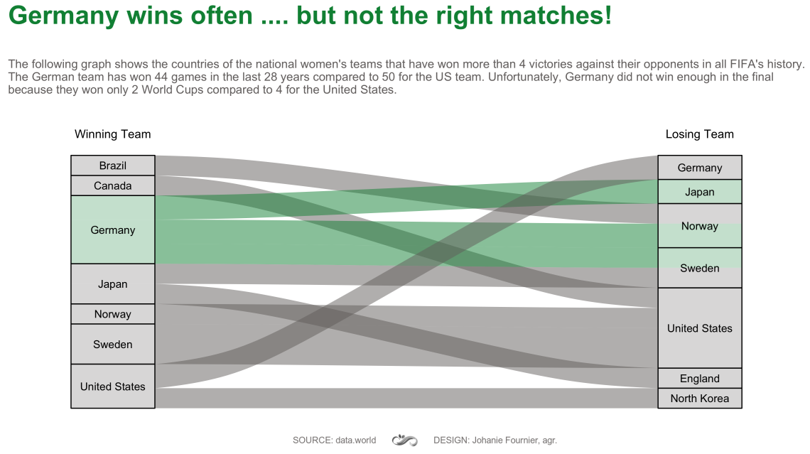
gg<-gg + labs(title="Germany wins often .... but not the right matches!\n",
              subtitle="The following graph shows the countries of the national women's teams that have won more than 4 victories against their opponents in all FIFA's history.\nThe German team has won 44 games in the last 28 years compared to 50 for the US team. Unfortunately, Germany did not win enough in the final\nbecause they won only 2 World Cups compared to 4 for the United States.\n\n",
             y=" ", 
              x=" ")
gg<-gg + theme(plot.title    = element_text(hjust=0,size=26, color="#018E42", face="bold"),
                plot.subtitle = element_text(hjust=0,size=12, color="#736F6E"),
               axis.title.y  = element_blank(),
               axis.title.x  = element_blank(),
               axis.text.y   = element_blank(), 
               axis.text.x   = element_text(hjust=0.5, size=12, color="#000000"))